Getting started#
The main modelling routine is empymod.model.bipole, which can compute
the electromagnetic frequency- or time-domain field due to arbitrary finite
electric or magnetic dipole sources, measured by arbitrary finite electric or
magnetic dipole receivers. The model is defined by horizontal resistivity and
anisotropy, horizontal and vertical electric permittivities and horizontal and
vertical magnetic permeabilities. By default, the electromagnetic response is
normalized to source and receiver of 1 m length, and source strength of 1 A.
Basic example#
A simple frequency-domain example, where we keep most of the parameters left at the default value:
In [1]: import empymod
   ...: import numpy as np
   ...: import matplotlib.pyplot as plt
   ...:
First we define the survey parameters: source and receiver locations, and source frequencies.
In [2]: # x-directed dipole source: x0, x1, y0, y1, z0, z1
   ...: source = [-50, 50, 0, 0, -100, -100]
   ...: # Source frequency
   ...: frequency = 1
   ...: # Receiver offsets
   ...: offsets = np.arange(1, 11)*500
   ...: # x-directed dipole receiver-array: x, y, z, azimuth, dip
   ...: receivers = [offsets, offsets*0, -200, 0, 0]
   ...:
Next, we define the resistivity model:
In [3]: # Layer boundaries
   ...: depth = [0, -300, -1000, -1050]
   ...: # Layer resistivities
   ...: resistivities = [1e20, 0.3, 1, 50, 1]
   ...:
And finally we compute the electromagnetic response at receiver locations:
In [4]: efield = empymod.bipole(
   ...:         src=source,
   ...:         rec=receivers,
   ...:         depth=depth,
   ...:         res=resistivities,
   ...:         freqtime=frequency,
   ...:         verb=4,
   ...: )
   ...:

:: empymod START  ::  v2.6.1.dev1+gd9bfeebfc

   depth       [m] :  -1050 -1000 -300 0
   res     [Ohm.m] :  1 50 1 0.3 1E+20
   aniso       [-] :  1 1 1 1 1
   epermH      [-] :  1 1 1 1 1
   epermV      [-] :  1 1 1 1 1
   mpermH      [-] :  1 1 1 1 1
   mpermV      [-] :  1 1 1 1 1
   direct field    :  Comp. in wavenumber domain
   frequency  [Hz] :  1
   Hankel          :  DLF (Fast Hankel Transform)
     > Filter      :  key_201_2009
     > DLF type    :  Standard
   Loop over       :  None (all vectorized)
   Source type     :  Electric field
   Receiver type   :  Electric field
   Source(s)       :  1 dipole(s)
     > intpts      :  1 (as dipole)
     > length  [m] :  100
     > strength[A] :  0
     > x_c     [m] :  0
     > y_c     [m] :  0
     > z_c     [m] :  -100
     > azimuth [°] :  0
     > dip     [°] :  0
   Receiver(s)     :  10 dipole(s)
     > x       [m] :  500 - 5000 : 10  [min-max; #]
                   :  500 1000 1500 2000 2500 3000 3500 4000 4500 5000
     > y       [m] :  0 - 0 : 10  [min-max; #]
                   :  0 0 0 0 0 0 0 0 0 0
     > z       [m] :  -200
     > azimuth [°] :  0
     > dip     [°] :  0
   Required ab's   :  11

:: empymod END; runtime = 0:00:00.003314 :: 1 kernel call(s)
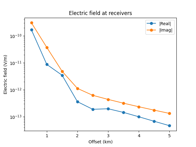
Let’s plot the resulting responses:
In [5]: fig, ax = plt.subplots()
   ...: ax.semilogy(offsets/1e3, abs(efield.real), 'C0o-', label='|Real|')
   ...: ax.semilogy(offsets/1e3, abs(efield.imag), 'C1o-', label='|Imag|')
   ...: ax.legend()
   ...: ax.set_title('Electric field at receivers')
   ...: ax.set_xlabel('Offset (km)');
   ...: ax.set_ylabel('Electric field (V/m)');
   ...:
A good starting point is the Gallery-gallery or [Wert17b], and
more detailed information can be found in [Wert17]. The description of all
parameters can be found in the API documentation for
empymod.model.bipole.
Structure#
The structure of empymod is:
model.py: EM modelling; principal end-user facing routines.
utils.py: Utilities such as checking input parameters.
kernel.py: Kernel of empymod, computes the wavenumber-domain electromagnetic response. Plus analytical, frequency-domain full- and half-space solutions.
transform.py: Methods to carry out the required Hankel transform from wavenumber to space domain and Fourier transform from frequency to time domain.
filters.py: Filters for the Digital Linear Filters method DLF (Hankel and Fourier transforms).
Coordinate system#
The used coordinate system is either a
Left-Handed System (LHS), where Easting is the \(x\)-direction, Northing the \(y\)-direction, and positive \(z\) is pointing downwards;
Right-Handed System (RHS), where Easting is the \(x\)-direction, Northing the \(y\)-direction, and positive \(z\) is pointing upwards.
Have a look at the example Definition of the coordinate system in empymod for further explanations.
Theory#
The code is principally based on
[HuTS15] for the wavenumber-domain computation (
kernel),[Key12] for the DLF and QWE transforms,
[SlHM10] for the analytical half-space solutions, and
[Hami00] for the FFTLog.
See these publications and all the others given in the References, if you are interested in the theory on which empymod is based. Another good reference is [ZiSl19]. The book derives in great detail the equations for layered-Earth CSEM modelling.