Coordinate system

Short version

The used coordinate system is either a

• Left-Handed System (LHS), where Easting is the \(x\)-direction, Northing the \(y\)-direction, and positive \(z\) is pointing downwards;
• Right-Handed System (RHS), where Easting is the \(x\)-direction, Northing the \(y\)-direction, and positive \(z\) is pointing upwards.

In more detail

The derivation on which empymod is based ([HuTS15]) uses a right-handed system with \(x\) to the East, \(y\) to the South, and \(z\) downwards (ESD). In the actual original implementation of empymod this was changed to a left-handed system with \(x\) to the East, \(y\) to the North, and \(z\) downwards (END). However, empymod can equally well be used for a coordinate system where positive \(z\) is pointing up by just flipping \(z\), resulting in \(x\) to the East, \(y\) to the North, and \(z\) upwards (ENU).

	Left-handed system	Right-handed system
\(x\)	Easting	Easting
\(y\)	Northing	Northing
\(z\)	Down	Up
\(\theta\)	Angle E-N	Angle E-N
\(\varphi\)	Angle down	Angle up

There are a few other important points to keep in mind when switching between coordinate systems:

• The interfaces (depth) have to be defined continuously increasing or decreasing, either from lowest to highest or the other way around. E.g., a simple five-layer model with the sea-surface at 0 m, a 100 m water column, and a target of 50 m 900 m below the seafloor can be defined in four ways:

  • [0, 100, 1000, 1050] -> LHS low to high
  • [0, -100, -1000, -1050] -> RHS high to low
  • [1050, 1000, 100, 0] -> LHS high to low
  • [-1050, -1000, -100, 0] -> RHS low to high

• The above point affects also all model parameters (res, aniso, {e;m}perm{H;V}). E.g., for the above five-layer example this would be

  • res = [1e12, 0.3, 1, 50, 1] -> LHS low to high
  • res = [1e12, 0.3, 1, 50, 1] -> RHS high to low
  • res = [1, 50, 1, 0.3, 1e12] -> LHS high to low
  • res = [1, 50, 1, 0.3, 1e12] -> RHS low to high

  Note that in a two-layer scenario the values are always taken as low-to-high (as it is not possible to detect the direction from only one interface).

• A source or a receiver exactly on a boundary is taken as being in the lower layer. Hence, if \(z_\rm{rec} = z_0\), where \(z_0\) is the surface, then the receiver is taken as in the air in the LHS, but as in the subsurface in the RHS. Similarly, if \(z_\rm{rec} = z_\rm{seafloor}\), then the receiver is taken as in the sea in the LHS, but as in the subsurface in the RHS. This can be avoided by never placing it exactly on a boundary, but slightly (e.g., 1 mm) in the layer where you want to have it.

• In bipole, the dip switches sign. Correspondingly in dipole, the ab’s containing vertical directions switch the sign for each vertical component.

• Sign switches also occur for magnetic sources or receivers.

In this example we first create a sketch of the LHS and RHS for visualization, followed by a few examples using dipole and bipole to demonstrate the two possibilities.

import empymod
import numpy as np
import matplotlib.pyplot as plt
from mpl_toolkits.mplot3d import Axes3D
from mpl_toolkits.mplot3d import proj3d
from matplotlib.patches import FancyArrowPatch
plt.style.use('ggplot')

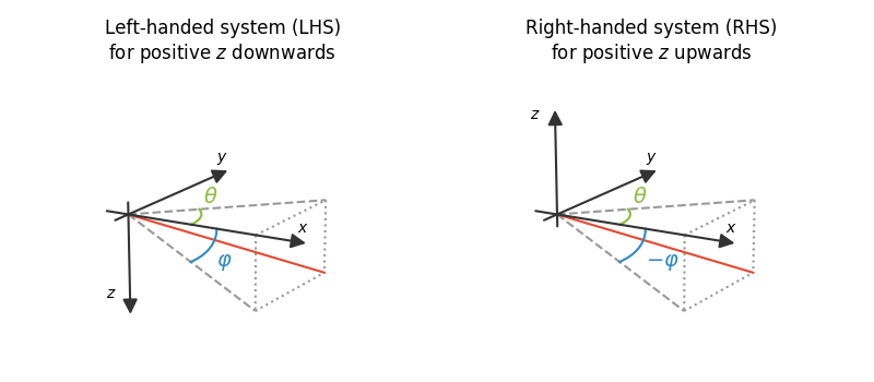
RHS vs LHS

Comparison of the right-handed system with positive \(z\) downwards and the left-handed system with positive \(z\) upwards. Easting is always \(x\), and Northing is \(y\).

class Arrow3D(FancyArrowPatch):
    """https://stackoverflow.com/a/29188796"""

    def __init__(self, xs, ys, zs):
        FancyArrowPatch.__init__(
                self, (0, 0), (0, 0), mutation_scale=20, lw=1.5,
                arrowstyle='-|>', color='.2', zorder=100)
        self._verts3d = xs, ys, zs

    def draw(self, renderer):
        xs3d, ys3d, zs3d = self._verts3d
        xs, ys, _ = proj3d.proj_transform(xs3d, ys3d, zs3d, renderer.M)
        self.set_positions((xs[0], ys[0]), (xs[1], ys[1]))
        FancyArrowPatch.draw(self, renderer)

def repeated(ax, pm):
    """These are all repeated for the two subplots."""

    # Coordinate system
    # The first three are not visible, but for the aspect ratio of the plot.
    ax.plot([-2, 12], [0, 0], [0, 0], c='w')
    ax.plot([0, 0], [-2, 12], [0, 0], c='w')
    ax.plot([0, 0], [0, 0], [-pm*2, pm*12], c='w')
    ax.add_artist(Arrow3D([-2, 14], [0, 0], [0, 0]))
    ax.add_artist(Arrow3D([0, 0], [-2, 14], [0, 0]))
    ax.add_artist(Arrow3D([0, 0], [0, 0], [-pm*2, pm*14]))

    # Annotate it
    ax.text(12, 2, 0, r'$x$')
    ax.text(0, 12, 2, r'$y$')
    ax.text(-2, 0, pm*12, r'$z$')

    # Helper lines
    ax.plot([0, 10], [0, 10], [0, 0], '--', c='.6')
    ax.plot([0, 10], [0, 0], [0, -10], '--', c='.6')
    ax.plot([10, 10], [0, 10], [0, 0], ':', c='.6')
    ax.plot([10, 10], [10, 10], [0, -10], ':', c='.6')
    ax.plot([10, 10], [0, 0], [0, -10], ':', c='.6')
    ax.plot([10, 10], [0, 10], [-10, -10], ':', c='.6')

    # Resulting trajectory
    ax.plot([0, 10], [0, 10], [0, -10], 'C0')

    # Theta
    azimuth = np.linspace(np.pi/4, np.pi/2, 31)
    ax.plot(np.sin(azimuth)*5, np.cos(azimuth)*5, 0, c='C5')
    ax.text(3, 5, 0, r"$\theta$", color='C5', fontsize=14)

    # Phi
    ax.plot(np.sin(azimuth)*7, azimuth*0, -np.cos(azimuth)*7, c='C1')

    ax.view_init(azim=-60, elev=20)

# Create figure
fig = plt.figure(figsize=(8, 3.5))

# Left-handed system
ax1 = fig.add_subplot(121, projection=Axes3D.name, facecolor='w')
ax1.axis('off')
plt.title('Left-handed system (LHS)\nfor positive $z$ downwards', fontsize=12)
ax1.text(7, 0, -5, r"$\varphi$", color='C1', fontsize=14)

repeated(ax1, -1)

# Right-handed  system
ax2 = fig.add_subplot(122, projection='3d', facecolor='w', sharez=ax1)
ax2.axis('off')
plt.title('Right-handed system (RHS)\nfor positive $z$ upwards', fontsize=12)
ax2.text(7, 0, -5, r"$-\varphi$", color='C1', fontsize=14)

repeated(ax2, 1)

plt.tight_layout()
plt.show()

Dipole

A simple example using dipole. It is a marine case with 300 meter water depth and a 50 m thick target 700 m below the seafloor.

off = np.linspace(500, 10000, 301)

LHS

In the left-handed system positive \(z\) is downwards. So we have to define our model by beginning with the air layer, followed by water, background, target, and background again. This means that all our depth-values are positive, as the air-interface \(z_0\) is at 0 m.

lhs = empymod.dipole(
        src=[0, 0, 100],
        rec=[off, np.zeros(off.size), 200],
        depth=[0, 300, 1000, 1050],
        res=[1e20, 0.3, 1, 50, 1],
        # depth=[1050, 1000, 300, 0],  # Alternative way, LHS high to low.
        # res=[1, 50, 1, 0.3, 1e20],   # " " "
        freqtime=1,
        verb=0
)

RHS

In the right-handed system positive \(z\) is upwards. So we have to define our model by beginning with the background, followed by the target, background again, water, and air. This means that all our depth-values are negative.

rhs = empymod.dipole(
        src=[0, 0, -100],
        rec=[off, np.zeros(off.size), -200],
        depth=[0, -300, -1000, -1050],
        res=[1e20, 0.3, 1, 50, 1],
        # depth=[-1050, -1000, -300, 0],  # Alternative way, RHS low to high.
        # res=[1, 50, 1, 0.3, 1e20],      # " " "
        freqtime=1,
        verb=0
)

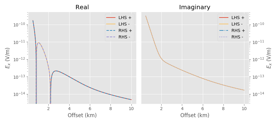
Compare

Plotting the two confirms that the results agree, no matter if we use the LHS or the RHS definition.

plt.figure(figsize=(9, 4))

ax1 = plt.subplot(121)
plt.title('Real')
plt.plot(off/1e3, lhs.real, 'C0', label='LHS +')
plt.plot(off/1e3, -lhs.real, 'C4', label='LHS -')
plt.plot(off/1e3, rhs.real, 'C1--', label='RHS +')
plt.plot(off/1e3, -rhs.real, 'C2--', label='RHS -')
plt.yscale('log')
plt.xlabel('Offset (km)')
plt.ylabel('$E_x$ (V/m)')
plt.legend()

ax2 = plt.subplot(122, sharey=ax1)
plt.title('Imaginary')
plt.plot(off/1e3, lhs.imag, 'C0', label='LHS +')
plt.plot(off/1e3, -lhs.imag, 'C4', label='LHS -')
plt.plot(off/1e3, rhs.imag, 'C1-.', label='RHS +')
plt.plot(off/1e3, -rhs.imag, 'C2:', label='RHS -')
plt.yscale('log')
plt.xlabel('Offset (km)')
plt.ylabel('$E_x$ (V/m)')
plt.legend()
ax2.yaxis.set_label_position("right")
ax2.yaxis.tick_right()

plt.tight_layout()
plt.show()

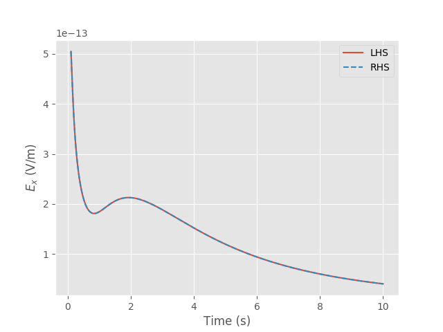
Bipole [x1, x2, y1, y2, z1, z2]

A time-domain example using rotated bipoles, where we define them as \([x_1, x_2, y_1, y_2, z_1, z_2]\).

times = np.linspace(0.1, 10, 301)
inp = {'freqtime': times, 'signal': 0, 'verb': 0}

lhs = empymod.bipole(
        src=[-50, 50, -10, 10, 100, 110],
        rec=[6000, 6100, 20, -20, 220, 200],
        depth=[0, 300, 1000, 1050],
        res=[1e20, 0.3, 1, 50, 1],
        **inp
)

rhs = empymod.bipole(
        src=[-50, 50, -10, 10, -100, -110],
        rec=[6000, 6100, 20, -20, -220, -200],
        depth=[0, -300, -1000, -1050],
        res=[1e20, 0.3, 1, 50, 1],
        **inp
)

plt.figure()

plt.plot(times, lhs, 'C0', label='LHS')
plt.plot(times, rhs, 'C1--', label='RHS')
plt.xlabel('Time (s)')
plt.ylabel('$E_x$ (V/m)')
plt.legend()

plt.show()

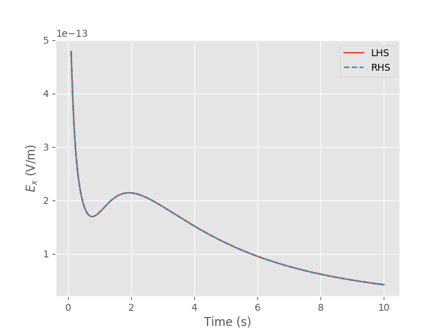
Bipole [x, y, z, azimuth, dip]

A very similar time-domain example using rotated bipoles, but this time defining them as \([x, y, z, \theta, \varphi]\). Note that \(\varphi\) has to change the sign, while \(\theta\) does not.

lhs = empymod.bipole(
        src=[0, 0, 100, 10, 20],
        rec=[6000, 0, 200, -5, 15],
        depth=[0, 300, 1000, 1050],
        res=[1e20, 0.3, 1, 50, 1],
        **inp
)

rhs = empymod.bipole(
        src=[0, 0, -100, 10, -20],
        rec=[6000, 0, -200, -5, -15],
        depth=[0, -300, -1000, -1050],
        res=[1e20, 0.3, 1, 50, 1],
        **inp
)

plt.figure()

plt.plot(times, lhs, 'C0', label='LHS')
plt.plot(times, rhs, 'C1--', label='RHS')
plt.xlabel('Time (s)')
plt.ylabel('$E_x$ (V/m)')
plt.legend()

plt.show()

empymod.Report()

Estimated memory usage: 43 MB