Note
Click here to download the full example code
Transform utilities within empymod for other modellers
This is an example how you can use the Fourier-transform tools implemented in
empymod with other modellers. You could achieve the same for the Hankel
transform.
empymod has various Fourier transforms implemented:
Digital Linear Filters DLF (Sine/Cosine)
Quadrature with Extrapolation QWE
Logarithmic Fast Fourier Transform FFTLog
Fast Fourier Transform FFT
For details of all the parameters see the empymod-docs or the function’s
docstrings.
import empymod
import numpy as np
import matplotlib.pyplot as plt
plt.style.use('ggplot')
Model and transform parameters
The model actually doesn’t matter for our purpose, but we need some model to show how it works.
# Define model, a halfspace
model = {
    'src': [0, 0, 0.001],     # Source at origin, slightly below interface
    'rec': [6000, 0, 0.001],  # Receivers in-line, 0.5m below interface
    'depth': [0],             # Air interface
    'res': [2e14, 1],         # Resistivity: [air, half-space]
    'epermH': [0, 1],         # Set el. perm. of air to 0 because of num. noise
}

# Specify desired times
time = np.linspace(0.1, 30, 301)

# Desired time-domain signal (0: impulse; 1: step-on; -1: step-off)
signal = 1

# Get required frequencies to model this time-domain result
# => we later need ``ft`` and ``ftarg`` for the Fourier transform.
# => See the docstrings (e.g., empymod.model.dipole) for available transforms
#    and their arguments.
time, freq, ft, ftarg = empymod.utils.check_time(
        time=time, signal=signal, ft='dlf', ftarg={}, verb=3)
Out:
time        [s] :  0.1 - 30 : 301  [min-max; #]
Fourier         :  DLF (Sine-Filter)
  > Filter      :  Key 201 CosSin (2012)
  > DLF type    :  Lagged Convolution
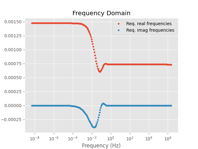
Frequency-domain computation
=> Here we compute the frequency-domain result with `empymod`, but you could compute it with any other modeller.
fresp = empymod.dipole(freqtime=freq, **model)
Out:
:: empymod END; runtime = 0:00:00.029106 :: 1 kernel call(s)
Plot frequency-domain result
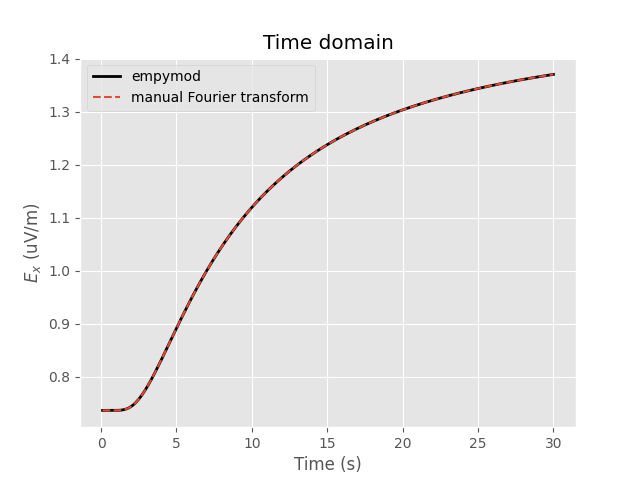
Fourier transform
# Compute corresponding time-domain signal.
tresp, _ = empymod.model.tem(
    fEM=fresp[:, None],
    off=np.array(model['rec'][0]),
    freq=freq,
    time=time,
    signal=signal,
    ft=ft,
    ftarg=ftarg)

tresp = np.squeeze(tresp)

# Time-domain result just using empymod
tresp2 = empymod.dipole(freqtime=time, signal=signal, verb=1, **model)
Plot time-domain result
empymod.Report()
Total running time of the script: ( 0 minutes 1.828 seconds)
Estimated memory usage: 9 MB