Note
Click here to download the full example code
Step and impulse responses
These examples compare the analytical solution with empymod for time-domain step and impulse responses for inline, x-directed source and receivers, for the four different frequency-to-time methods QWE, DLF, FFTLog, and FFT. Which method is faster and which is more precise depends on the model (land or marine, source/receiver at air-interface or not) and the response (step or impulse).
import empymod
import numpy as np
from scipy.special import erf
import matplotlib.pyplot as plt
from scipy.constants import mu_0       # Permeability of free space  [H/m]
plt.style.use('ggplot')
colors = [color['color'] for color in list(plt.rcParams['axes.prop_cycle'])]
Analytical solutions
Analytical solution for source and receiver at the interface between two half-spaces
The time-domain step and impulse responses for a source at the origin (\(x_s = y_s = z_s = 0\) m) and an in-line receiver at the surface (\(y_r = z_r = 0\) m), is given by the following equations, where \(\rho_h\) is horizontal resistivity (\(\Omega\) m), \(\lambda\) is anisotropy (-), with \(\lambda = \sqrt{\rho_v/\rho_h}\), \(r\) is offset (m), \(t\) is time (s), and \(\tau_h = \sqrt{\mu_0 r^2/(\rho_h t)}\); \(\mu_0\) is the magnetic permeability of free space (H/m).
Time Domain: Step Response \(\mathbf{\mathcal{H}(t)}\)
Time Domain: Impulse Response \(\mathbf{\delta(t)}\)
Reference
Equations 3.2 and 3.3 in Werthmüller, D., 2009, Inversion of multi-transient EM data from anisotropic media: M.S. thesis, TU Delft, ETH Zürich, RWTH Aachen; UUID: f4b071c1-8e55-4ec5-86c6-a2d54c3eda5a.
Analytical functions
def ee_xx_impulse(res, aniso, off, time):
    """VTI-Halfspace impulse response, xx, inline.

    res   : horizontal resistivity [Ohm.m]
    aniso : anisotropy [-]
    off   : offset [m]
    time  : time(s) [s]
    """
    tau_h = np.sqrt(mu_0*off**2/(res*time))
    t0 = tau_h/(2*time*np.sqrt(np.pi))
    t1 = np.exp(-tau_h**2/4)
    t2 = tau_h**2/(2*aniso**2) + 1
    t3 = np.exp(-tau_h**2/(4*aniso**2))
    Exx = res/(2*np.pi*off**3)*t0*(-t1 + t2*t3)
    Exx[time == 0] = res/(2*np.pi*off**3)  # Delta dirac part
    return Exx


def ee_xx_step(res, aniso, off, time):
    """VTI-Halfspace step response, xx, inline.

    res   : horizontal resistivity [Ohm.m]
    aniso : anisotropy [-]
    off   : offset [m]
    time  : time(s) [s]
    """
    tau_h = np.sqrt(mu_0*off**2/(res*time))
    t0 = erf(tau_h/2)
    t1 = 2*aniso*erf(tau_h/(2*aniso))
    t2 = tau_h/np.sqrt(np.pi)*np.exp(-tau_h**2/(4*aniso**2))
    Exx = res/(2*np.pi*off**3)*(2*aniso + t0 - t1 + t2)
    return Exx
Example 1: Source and receiver at z=0m
Comparison with analytical solution; put 1 mm below the interface, as they would be regarded as in the air by emmod otherwise.
src = [0, 0, 0.001]          # Source at origin, slightly below interface
rec = [6000, 0, 0.001]       # Receivers in-line, 0.5m below interface
res = [2e14, 10]             # Resistivity: [air, half-space]
aniso = [1, 2]               # Anisotropy: [air, half-space]
eperm = [0, 1]               # Set el. perm. of air to 0 because of num. noise
t = np.logspace(-2, 1, 301)  # Desired times (s)

# Collect parameters
inparg = {'src': src, 'rec': rec, 'depth': 0, 'freqtime': t, 'res': res,
          'aniso': aniso, 'epermH': eperm, 'ht': 'dlf', 'verb': 2}
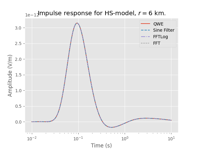
Impulse response
ex = ee_xx_impulse(res[1], aniso[1], rec[0], t)

inparg['signal'] = 0  # signal 0 = impulse
print('QWE')
qwe = empymod.dipole(**inparg, ft='qwe')
print('DLF (Sine)')
sin = empymod.dipole(**inparg, ft='dlf', ftarg={'dlf': 'key_81_CosSin_2009'})
print('FFTLog')
ftl = empymod.dipole(**inparg, ft='fftlog')
print('FFT')
fft = empymod.dipole(
        **inparg, ft='fft',
        ftarg={'dfreq': .0005, 'nfreq': 2**20, 'pts_per_dec': 10})
Out:
QWE
* WARNING :: Fourier-quadrature did not converge at least once;
             => desired `atol` and `rtol` might not be achieved.

:: empymod END; runtime = 0:00:03.563895 :: 1 kernel call(s)

DLF (Sine)

:: empymod END; runtime = 0:00:00.012587 :: 1 kernel call(s)

FFTLog

:: empymod END; runtime = 0:00:00.006852 :: 1 kernel call(s)

FFT

:: empymod END; runtime = 0:00:00.651102 :: 1 kernel call(s)
=> FFTLog is the fastest by quite a margin, followed by the Sine-filter. What cannot see from the output (set verb to something bigger than 2 to see it) is how many frequencies each method used:
QWE: 159 (0.000794328 - 63095.7 Hz)
Sine: 116 (5.33905E-06 - 52028 Hz)
FFTLog: 60 (0.000178575 - 141.847 Hz)
FFT: 61 (0.0005 - 524.288 Hz)
Note that for the actual transform, FFT used 2^20 = 1’048’576 frequencies! It only computed 60 frequencies, and then interpolated the rest, as it requires regularly spaced data.
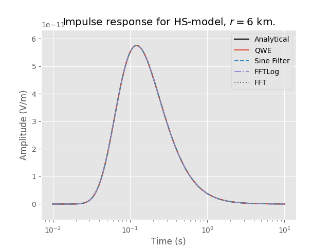
plt.figure()
plt.title(r'Impulse response for HS-model, $r=$' +
          str(int(rec[0]/1000)) + ' km.')
plt.xlabel('Time (s)')
plt.ylabel(r'Amplitude (V/m)')
plt.semilogx(t, ex, 'k-', label='Analytical')
plt.semilogx(t, qwe, 'C0-', label='QWE')
plt.semilogx(t, sin, 'C1--', label='Sine Filter')
plt.semilogx(t, ftl, 'C2-.', label='FFTLog')
plt.semilogx(t, fft, 'C3:', label='FFT')
plt.legend(loc='best')
plt.ylim([-.1*np.max(ex), 1.1*np.max(ex)])
plt.show()
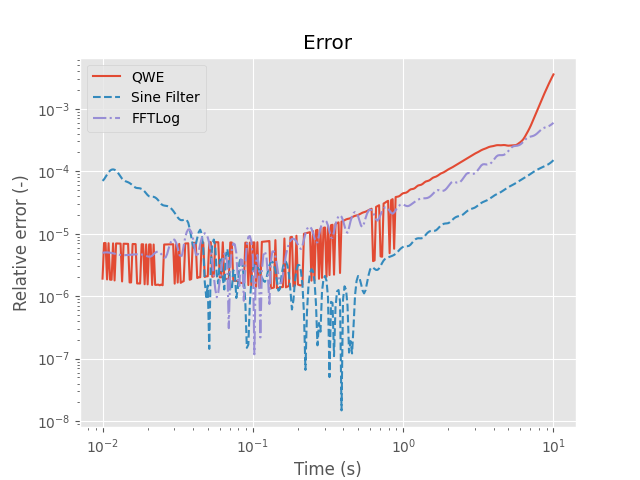
plt.figure()
plt.title('Error')
plt.xlabel('Time (s)')
plt.ylabel('Relative error (-)')
plt.loglog(t, abs(qwe-ex)/ex, 'C0-', label='QWE')
plt.plot(t, abs(sin-ex)/ex, 'C1--', label='Sine Filter')
plt.plot(t, abs(ftl-ex)/ex, 'C2-.', label='FFTLog')
plt.plot(t, abs(fft-ex)/ex, 'C3:', label='FFT')
plt.legend(loc='best')
plt.show()
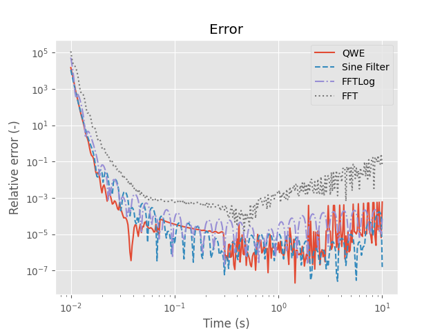
=> The error is comparable in all cases. FFT is not too good at later times. This could be improved by computing lower frequencies. But because FFT needs regularly spaced data, our vector would soon explode (and you would need a lot of memory). In the current case we are already using 2^20 samples!
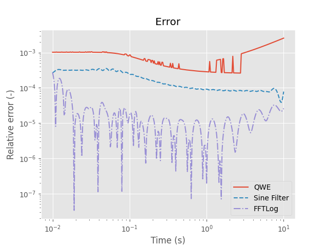
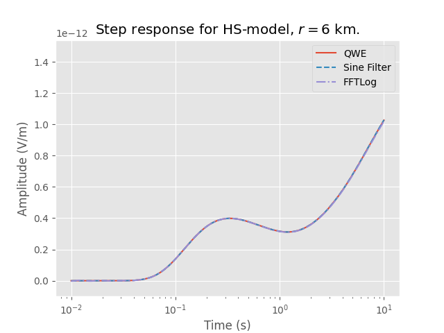
Step response
Step responses are almost impossible with FFT. We can either try to model late times with lots of low frequencies, or the step with lots of high frequencies. I do not use FFT in the step-response examples.
Switch-on
ex = ee_xx_step(res[1], aniso[1], rec[0], t)

inparg['signal'] = 1  # signal 1 = switch-on
print('QWE')
qwe = empymod.dipole(**inparg, ft='qwe')
print('DLF (Sine)')
sin = empymod.dipole(**inparg, ft='dlf', ftarg={'dlf': 'key_81_CosSin_2009'})
print('FFTLog')
ftl = empymod.dipole(**inparg, ft='fftlog', ftarg={'q': -0.6})
Out:
QWE
* WARNING :: Fourier-quadrature did not converge at least once;
             => desired `atol` and `rtol` might not be achieved.

:: empymod END; runtime = 0:00:14.868219 :: 1 kernel call(s)

DLF (Sine)

:: empymod END; runtime = 0:00:00.011536 :: 1 kernel call(s)

FFTLog

:: empymod END; runtime = 0:00:00.007358 :: 1 kernel call(s)
Used number of frequencies:
QWE: 159 (0.000794328 - 63095.7 Hz)
Sine: 116 (5.33905E-06 - 52028 Hz)
FFTLog: 60 (0.000178575 - 141.847 Hz)
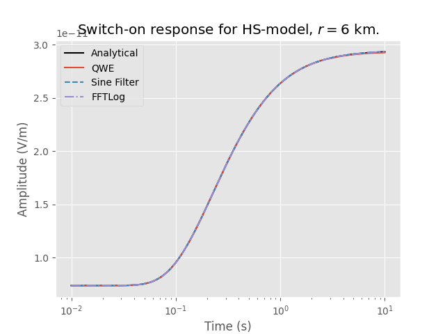
plt.figure()
plt.title(r'Switch-on response for HS-model, $r=$' +
          str(int(rec[0]/1000)) + ' km.')
plt.xlabel('Time (s)')
plt.ylabel('Amplitude (V/m)')
plt.semilogx(t, ex, 'k-', label='Analytical')
plt.semilogx(t, qwe, 'C0-', label='QWE')
plt.semilogx(t, sin, 'C1--', label='Sine Filter')
plt.semilogx(t, ftl, 'C2-.', label='FFTLog')
plt.legend(loc='best')
plt.show()
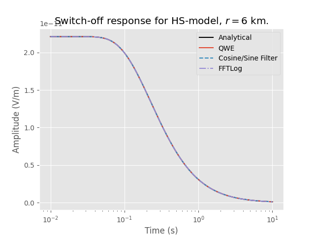
Switch-off
For switch-off to work properly you need empymod-version bigger than 1.3.0! You can do it with previous releases too, but you will have to do the DC-computation and subtraction manually, as is done here for ee_xx_step.
exDC = ee_xx_step(res[1], aniso[1], rec[0], 60*60)
ex = exDC - ee_xx_step(res[1], aniso[1], rec[0], t)

inparg['signal'] = -1  # signal -1 = switch-off
print('QWE')
qwe = empymod.dipole(**inparg, ft='qwe')
print('DLF (Cosine/Sine)')
sin = empymod.dipole(**inparg, ft='dlf', ftarg={'dlf': 'key_81_CosSin_2009'})
print('FFTLog')
ftl = empymod.dipole(**inparg, ft='fftlog', ftarg={'add_dec': [-5, 3]})
Out:
QWE
* WARNING :: Fourier-quadrature did not converge at least once;
             => desired `atol` and `rtol` might not be achieved.

:: empymod END; runtime = 0:00:11.102383 :: 1 kernel call(s)

DLF (Cosine/Sine)

:: empymod END; runtime = 0:00:00.011099 :: 1 kernel call(s)

FFTLog

:: empymod END; runtime = 0:00:00.009982 :: 1 kernel call(s)
plt.figure()
plt.title(r'Switch-off response for HS-model, $r=$' +
          str(int(rec[0]/1000)) + ' km.')
plt.xlabel('Time (s)')
plt.ylabel('Amplitude (V/m)')
plt.semilogx(t, ex, 'k-', label='Analytical')
plt.semilogx(t, qwe, 'C0-', label='QWE')
plt.semilogx(t, sin, 'C1--', label='Cosine/Sine Filter')
plt.semilogx(t, ftl, 'C2-.', label='FFTLog')
plt.legend(loc='best')
plt.show()
Example 2: Air-seawater-halfspace
In seawater the transformation is generally much easier, as we do not have the step or the impules at zero time.
src = [0, 0, 950]            # Source 50 m above seabottom
rec = [6000, 0, 1000]        # Receivers in-line, at seabottom
res = [1e23, 1/3, 10]        # Resistivity: [air, water, half-space]
aniso = [1, 1, 2]            # Anisotropy: [air, water, half-space]
t = np.logspace(-2, 1, 301)  # Desired times (s)

# Collect parameters
inparg = {'src': src, 'rec': rec, 'depth': [0, 1000], 'freqtime': t,
          'res': res, 'aniso': aniso, 'ht': 'dlf', 'verb': 2}
Impulse response
inparg['signal'] = 0  # signal 0 = impulse
print('QWE')
qwe = empymod.dipole(**inparg, ft='qwe', ftarg={'maxint': 500})
print('DLF (Sine)')
sin = empymod.dipole(**inparg, ft='dlf', ftarg={'dlf': 'key_81_CosSin_2009'})
print('FFTLog')
ftl = empymod.dipole(**inparg, ft='fftlog')
print('FFT')
fft = empymod.dipole(
        **inparg, ft='fft',
        ftarg={'dfreq': .001, 'nfreq': 2**15, 'ntot': 2**16, 'pts_per_dec': 10}
        )
Out:
QWE

:: empymod END; runtime = 0:00:15.954267 :: 1 kernel call(s)

DLF (Sine)

:: empymod END; runtime = 0:00:00.028780 :: 1 kernel call(s)

FFTLog

:: empymod END; runtime = 0:00:00.015054 :: 1 kernel call(s)

FFT

:: empymod END; runtime = 0:00:00.043588 :: 1 kernel call(s)
Used number of frequencies:
QWE: 167 (0.000794328 - 158489 Hz)
Sine: 116 (5.33905E-06 - 52028 Hz)
FFTLog: 60 (0.000178575 - 141.847 Hz)
FFT: 46 (0.001 - 32.768 Hz)
plt.figure()
plt.title(r'Impulse response for HS-model, $r=$' +
          str(int(rec[0]/1000)) + ' km.')
plt.xlabel('Time (s)')
plt.ylabel(r'Amplitude (V/m)')
plt.semilogx(t, qwe, 'C0-', label='QWE')
plt.semilogx(t, sin, 'C1--', label='Sine Filter')
plt.semilogx(t, ftl, 'C2-.', label='FFTLog')
plt.semilogx(t, fft, 'C3:', label='FFT')
plt.legend(loc='best')
plt.show()
Step response
inparg['signal'] = 1  # signal 1 = step
print('QWE')
qwe = empymod.dipole(**inparg, ft='qwe', ftarg={'nquad': 31, 'maxint': 500})
print('DLF (Sine)')
sin = empymod.dipole(**inparg, ft='dlf', ftarg={'dlf': 'key_81_CosSin_2009'})
print('FFTLog')
ftl = empymod.dipole(**inparg, ft='fftlog', ftarg={'add_dec': [-2, 4]})
Out:
QWE
* WARNING :: Fourier-quadrature did not converge at least once;
             => desired `atol` and `rtol` might not be achieved.

:: empymod END; runtime = 0:00:13.402237 :: 1 kernel call(s)

DLF (Sine)

:: empymod END; runtime = 0:00:00.028819 :: 1 kernel call(s)

FFTLog

:: empymod END; runtime = 0:00:00.023197 :: 1 kernel call(s)
Used number of frequencies:
QWE: 173 (0.000398107 - 158489 Hz)
Sine: 116 (5.33905E-06 - 52028 Hz)
FFTLog: 90 (0.000178575 - 141847 Hz)
plt.figure()
plt.title(r'Step response for HS-model, $r=$' + str(int(rec[0]/1000)) + ' km.')
plt.xlabel('Time (s)')
plt.ylabel('Amplitude (V/m)')
plt.semilogx(t, qwe, 'C0-', label='QWE')
plt.semilogx(t, sin, 'C1--', label='Sine Filter')
plt.semilogx(t, ftl, 'C2-.', label='FFTLog')
plt.ylim([-.1e-12, 1.5*qwe.max()])
plt.legend(loc='best')
plt.show()
empymod.Report()
Total running time of the script: ( 1 minutes 3.863 seconds)
Estimated memory usage: 315 MB