Transform utilities within empymod for other modellers

This is an example how you can use the Fourier-transform tools implemented in empymod with other modellers. You could achieve the same for the Hankel transform.

empymod has various Fourier transforms implemented:

• Digital Linear Filters DLF (Sine/Cosine)

• Quadrature with Extrapolation QWE

• Logarithmic Fast Fourier Transform FFTLog

• Fast Fourier Transform FFT

For details of all the parameters see the empymod-docs or the function’s docstrings.

import empymod
import numpy as np
import matplotlib.pyplot as plt
plt.style.use('ggplot')

Model and transform parameters

The model actually doesn’t matter for our purpose, but we need some model to show how it works.

# Define model, a halfspace
model = {
    'src': [0, 0, 0.001],     # Source at origin, slightly below interface
    'rec': [6000, 0, 0.001],  # Receivers in-line, 0.5m below interface
    'depth': [0],             # Air interface
    'res': [2e14, 1],         # Resistivity: [air, half-space]
    'epermH': [0, 1],         # Set el. perm. of air to 0 because of num. noise
}

# Specify desired times
time = np.linspace(0.1, 30, 301)

# Desired time-domain signal (0: impulse; 1: step-on; -1: step-off)
signal = 1

# Get required frequencies to model this time-domain result
# => we later need ``ft`` and ``ftarg`` for the Fourier transform.
# => See the docstrings (e.g., empymod.model.dipole) for available transforms
#    and their arguments.
time, freq, ft, ftarg = empymod.utils.check_time(
        time=time, signal=signal, ft='dlf', ftarg={}, verb=3)

time        [s] :  0.1 - 30 : 301  [min-max; #]
Fourier         :  DLF (Sine-Filter)
  > Filter      :  key_201_2012
  > DLF type    :  Lagged Convolution

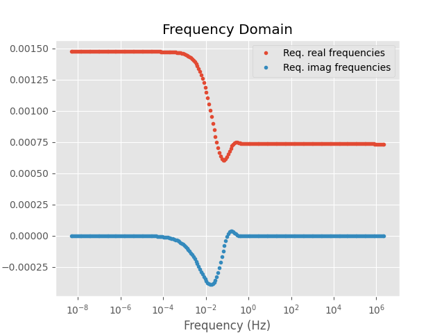
Frequency-domain computation

=> Here we compute the frequency-domain result with `empymod`, but you could compute it with any other modeller.

fresp = empymod.dipole(freqtime=freq, **model)

:: empymod END; runtime = 0:00:00.023251 :: 1 kernel call(s)

Plot frequency-domain result

plt.figure()

plt.title('Frequency Domain')
plt.plot(freq, 1e9*fresp.real, 'C0.', label='Req. real frequencies')
plt.plot(freq, 1e9*fresp.imag, 'C1.', label='Req. imag frequencies')
plt.legend()
plt.xscale('log')
plt.xlabel('Frequency (Hz)')
plt.ylabel('$E_x$ (nV/m)')

plt.show()

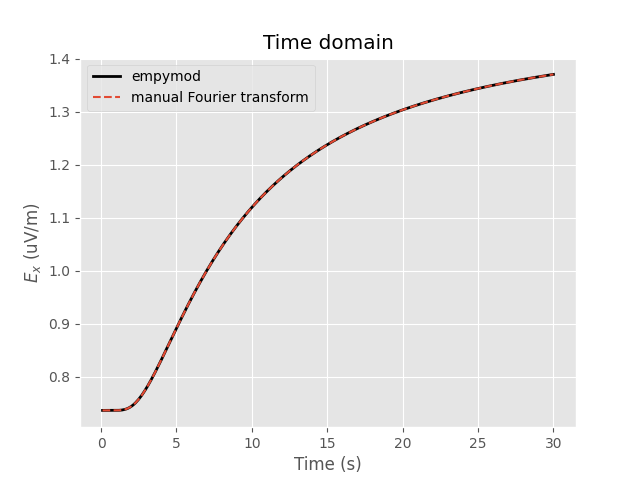
Fourier transform

# Compute corresponding time-domain signal.
tresp, _ = empymod.model.tem(
    fEM=fresp[:, None],
    off=np.array(model['rec'][0]),
    freq=freq,
    time=time,
    signal=signal,
    ft=ft,
    ftarg=ftarg)

tresp = np.squeeze(tresp)

# Time-domain result just using empymod
tresp2 = empymod.dipole(freqtime=time, signal=signal, verb=1, **model)

Plot time-domain result

fig = plt.figure()

plt.title('Time domain')
plt.plot(time, tresp2*1e12, 'k', lw=2, label='empymod')
plt.plot(time, tresp*1e12, 'C0--', label='manual Fourier transform')
plt.legend()
plt.xlabel('Time (s)')
plt.ylabel('$E_x$ (uV/m)')

plt.show()

empymod.Report()

Fri Mar 08 10:46:55 2024 UTC
OS	Linux	CPU(s)	2	Machine	x86_64
Architecture	64bit	RAM	7.5 GiB	Environment	Python
File system	ext4
Python 3.11.6 (main, Feb 1 2024, 16:47:41) [GCC 11.4.0]
numpy	1.26.4	scipy	1.12.0	numba	0.59.0
empymod	2.3.1.dev4+g0adb87d	libdlf	0.2.0	IPython	8.22.2
matplotlib	3.8.3

Estimated memory usage: 10 MB