Note
Go to the end to download the full example code.
Adding random noise to frequency-domain CSEM data#
Adding random noise to frequency-domain CSEM data is not a trivial task, and there are many different ways how it can be done. The problem comes from the fact that we live in the time domain, we do our measurements in the time domain, our noise is therefore time-domain noise, but we want to add complex-valued noise in the frequency domain.
Here we are going to look at some possibilities. However, keep in mind that there are more possibilities than the ones shown here.
1. Theory#
Let’s assume we have complex-valued data \(d=x+\text{i}y\). We can add random noise to the data in the following way,
where \(\tilde{d}\) is the data with added noise, \(\sigma\) is the standard deviation, \(\mu\) is the mean value of the randomly distributed noise, and \(\mathcal{R}\) is the random noise. We define the standard deviation as
where \(\epsilon_\text{n}\) is the noise floor and \(\epsilon_\text{r}\) is the relative error.
We compare here three ways of computing the random noise \(\mathcal{R}\). Of course there are other possibilities, e.g., one could make the non-zero mean a random realization itself.
Adding random uniform phases but constant amplitude
(3)#\[\mathcal{R}_\text{wn} = \exp[\text{i}\,\mathcal{U}(0, 2\pi)] \, ,\]where \(\mathcal{U}(0, 2\pi)\) is the uniform distribution and its range. This adds white noise with a flat amplitude spectrum and random phases.
Adding Gaussian noise to real and imaginary parts
Adding correlated random Gaussian noise
(4)#\[\mathcal{R}_\text{gc} = (1+\text{i})\,\mathcal{N}(0, 1) \, ,\]where \(\mathcal{N}(0, 1)\) is the standard normal distribution of zero mean and unit standard deviation.
Adding uncorrelated random Gaussian noise
Above is the correlated version. Noise could also be added completely uncorrelated,
(5)#\[\mathcal{R}_\text{gu} = \mathcal{N}(0, 1) + \text{i}\,\mathcal{N}(0, 1) \, .\]
import empymod
import numpy as np
import matplotlib.pyplot as plt
plt.style.use('bmh')
Noise computation#
# Initiate random number generator.
rng = np.random.default_rng()


def add_noise(data, ntype, rel_error, noise_floor, mu):
    """Add random noise to complex-valued data.

    If `ntype='white_noise'`, complex noise is generated from uniform randomly
    distributed phases.

    If `ntype='gaussian_correlated'`, correlated Gaussian random noise is added
    to real and imaginary part.

    If `ntype='gaussian_uncorrelated'`, uncorrelated Gaussian random noise is
    added to real and imaginary part.

    """

    # Standard deviation
    std = np.sqrt(noise_floor**2 + (rel_error*abs(data))**2)

    # Random noise
    if ntype == 'gaussian_correlated':
        noise = rng.standard_normal(data.size)*(1+1j)
    elif ntype == 'gaussian_uncorrelated':
        noise = 1j*rng.standard_normal(data.size)
        noise += rng.standard_normal(data.size)
    else:
        noise = np.exp(1j * rng.uniform(0, 2*np.pi, data.size))

    # Scale and move noise; add to data and return
    return data + std*((1+1j)*mu + noise)


def stack(n, data, ntype, **kwargs):
    """Stack n-times the noise, return normalized."""
    out = add_noise(data, ntype, **kwargs)/n
    for _ in range(n-1):
        out += add_noise(data, ntype, **kwargs)/n
    return out
2. Graphical illustration#
The following is a graphical illustration. Please note that the relative error is very high (20%)! This is only for illustration purposes.
# Inputs
d = np.array([6+2j])         # observed data point
mean = 0.3                   # Non-zero mean
relative_error = 0.2         # Very high relative error
std = relative_error*abs(d)  # std (without noise floor)

# Create figure
fig, axs = plt.subplots(2, 1, figsize=(8, 10), sharex=True, sharey=True)
ax1, ax2 = axs

# Titles
fig.suptitle(r"Random noise with $\epsilon_n = 0, "
             f"\\epsilon_r={relative_error}, \\mu={mean}$", y=1, fontsize=20)
ax1.set_title('Theoretical distributions')
ax2.set_title('Random realizations')

# Plot data point
for ax in axs:
    ax.plot(np.r_[0., d.real], np.r_[0., d.imag], '--', c='.5')
    ax.plot(d.real, d.imag, 'ko', ms=10, label='$d^{obs}$', zorder=10)


# Mean and standard deviation
ax1.plot(d.real+np.r_[0, std*mean], d.imag+np.r_[0, std*mean],
         'C8', label=r'Scaled mean $\sigma (1+i)\mu$', zorder=9)
ax1.plot(d.real+np.r_[std*mean, std*(1+mean)],
         d.imag+np.r_[std*mean, std*mean],
         'C1', label=r'Standard deviation $\sigma$')


# Random uniform phase
uniform_mean = std * ((1+1j)*mean + np.exp(1j*np.linspace(0, 2*np.pi, 301)))
ax1.plot(d.real+uniform_mean.real, d.imag+uniform_mean.imag,
         'C0', label='Random uniform phase')


# Gaussian
for i in range(1, 3):
    # Correlated
    ax1.plot(d.real + np.r_[-std, +std]*i + std*mean,
             d.imag + np.r_[-std, +std]*i + std*mean,
             'C3-', lw=6-2*i,
             label=f'Gaussian $\\pm {i} \\sigma$, correlated')

    # Uncorrelated
    ax1.plot(d.real + np.r_[-std, -std, +std, +std, -std]*i + std*mean,
             d.imag + np.r_[-std, +std, +std, -std, -std]*i + std*mean,
             'C2:', lw=6-2*i,
             label=f'Gaussian $\\pm {i} \\sigma$, uncorrelated')


# Plot random realizations
data = np.ones(300, dtype=complex)*d
shape = data.shape
rng = np.random.default_rng()
ls = ['C0x', 'C3+', 'C2x']
ntypes = ['white_noise', 'gaussian_correlated', 'gaussian_uncorrelated']
for i, ntype in enumerate(ntypes):

    # Add random noise of ntype.
    ndata = add_noise(data, ntype, relative_error, 0.0, mean)
    ax2.plot(ndata.real, ndata.imag, ls[i], label=ntype)


# Axis etc
for ax in axs:
    ax.axhline(c='k')
    ax.axvline(c='k')
    ax.legend(framealpha=1, loc='upper left')
    ax.set_aspect('equal')
    ax.set_ylabel('Imaginary part')
    ax.set_xlim([-4, 10])
ax2.set_xlabel('Real part')
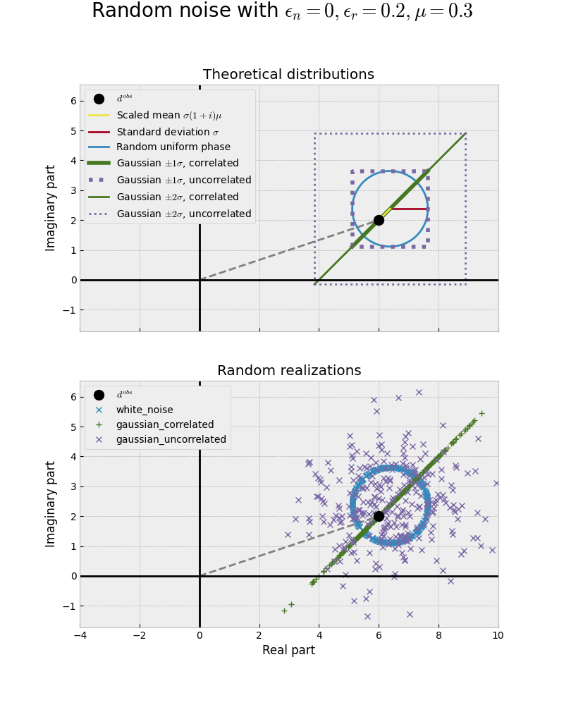
Intuitively one might think that the Gaussian uncorrelated noise is the “best” one, as it looks truly random. However, it is arguably the least “physical” one, as real and imaginary part of the electromagnetic field are not independent - if one changes, the other changes too. The uniformly distributed phases (blue circle) is the most physical noise corresponding to white noise adding random phases with a constant amplitude.
To get a better understanding we look at some numerical examples where we plot amplitude-vs-offset for a fixed frequency, and amplitude-vs-frequency for a fixed offset; for single realizations and when we stack it many times in order to reduce the noise.
3. Numerical examples#
Model#
# Model parameters
model = {
    'src': (0, 0, 0),  # Source at origin
    'depth': [],       # Homogenous space
    'res': 3,          # 3 Ohm.m
    'ab': 11,          # Ex-source, Ex-receiver}
}

# Single offset and offsets
offs = np.linspace(1000, 15000, 201)
off = 5000

# Single frequency and frequencies
freqs = np.logspace(-3, 2, 201)
freq = 1

# Responses
oresp = empymod.dipole(
    rec=(offs, offs*0, 0),  # Inline receivers
    freqtime=freq,
    **model
)
fresp = empymod.dipole(
    rec=(5000, 0, 0),     # Inline receiver
    freqtime=freqs,
    **model,
)

# Relative error, noise floor, mean of noise
rel_error = 0.05
noise_floor = 1e-15
n_stack = 1000

# Phase settings: wrapped, radians, lag-defined (+iw)
phase = {'unwrap': False, 'deg': False, 'lag': True}
:: empymod END; runtime = 0:00:00.006635 :: 1 kernel call(s)


:: empymod END; runtime = 0:00:00.003177 :: 1 kernel call(s)
Plotting function#
def error(resp, noise):
    """Return relative error (%) of noise with respect to resp."""
    return 100*abs((noise-resp)/resp)


def figure(x, data, reim, comp):
    fig, axs = plt.subplots(2, 4, constrained_layout=True,
                            figsize=(14, 8), sharex=True)

    axs[0, 0].set_title('|Real| (V/m)')
    axs[0, 0].plot(x, abs(data.real), 'k')
    axs[0, 0].plot(x, abs(reim.real), 'C0')
    axs[0, 0].plot(x, abs(comp.real), 'C1--')
    axs[0, 0].set_yscale('log')

    axs[1, 0].plot(x, error(data.real, reim.real), 'C0')
    axs[1, 0].plot(x, error(data.real, comp.real), 'C1--')
    axs[1, 0].set_ylabel('Rel. Error (%)')

    axs[0, 1].set_title('|Imaginary| (V/m)')
    axs[0, 1].plot(x, abs(data.imag), 'k', label='Data')
    axs[0, 1].plot(x, abs(reim.imag), 'C0', label='Noise to Re; Im')
    axs[0, 1].plot(x, abs(comp.imag), 'C1--', label='Noise to Complex')
    axs[0, 1].set_yscale('log')
    axs[0, 1].legend(fontsize=12, framealpha=1)

    axs[1, 1].plot(x, error(data.imag, reim.imag), 'C0')
    axs[1, 1].plot(x, error(data.imag, comp.imag), 'C1--')

    axs[0, 2].set_title('Amplitude (V/m)')
    axs[0, 2].plot(x, data.amp(), 'k')
    axs[0, 2].plot(x, reim.amp(), 'C0')
    axs[0, 2].plot(x, comp.amp(), 'C1--')
    axs[0, 2].set_yscale('log')

    axs[1, 2].plot(x, error(data.amp(), reim.amp()), 'C0')
    axs[1, 2].plot(x, error(data.amp(), comp.amp()), 'C1--')

    axs[0, 3].set_title('Phase (rad)')
    axs[0, 3].plot(x, data.pha(**phase), 'k')
    axs[0, 3].plot(x, reim.pha(**phase), 'C0')
    axs[0, 3].plot(x, comp.pha(**phase), 'C1--')

    axs[1, 3].plot(x, error(data.pha(**phase), reim.pha(**phase)), 'C0')
    axs[1, 3].plot(x, error(data.pha(**phase), comp.pha(**phase)), 'C1--')

    return fig, axs
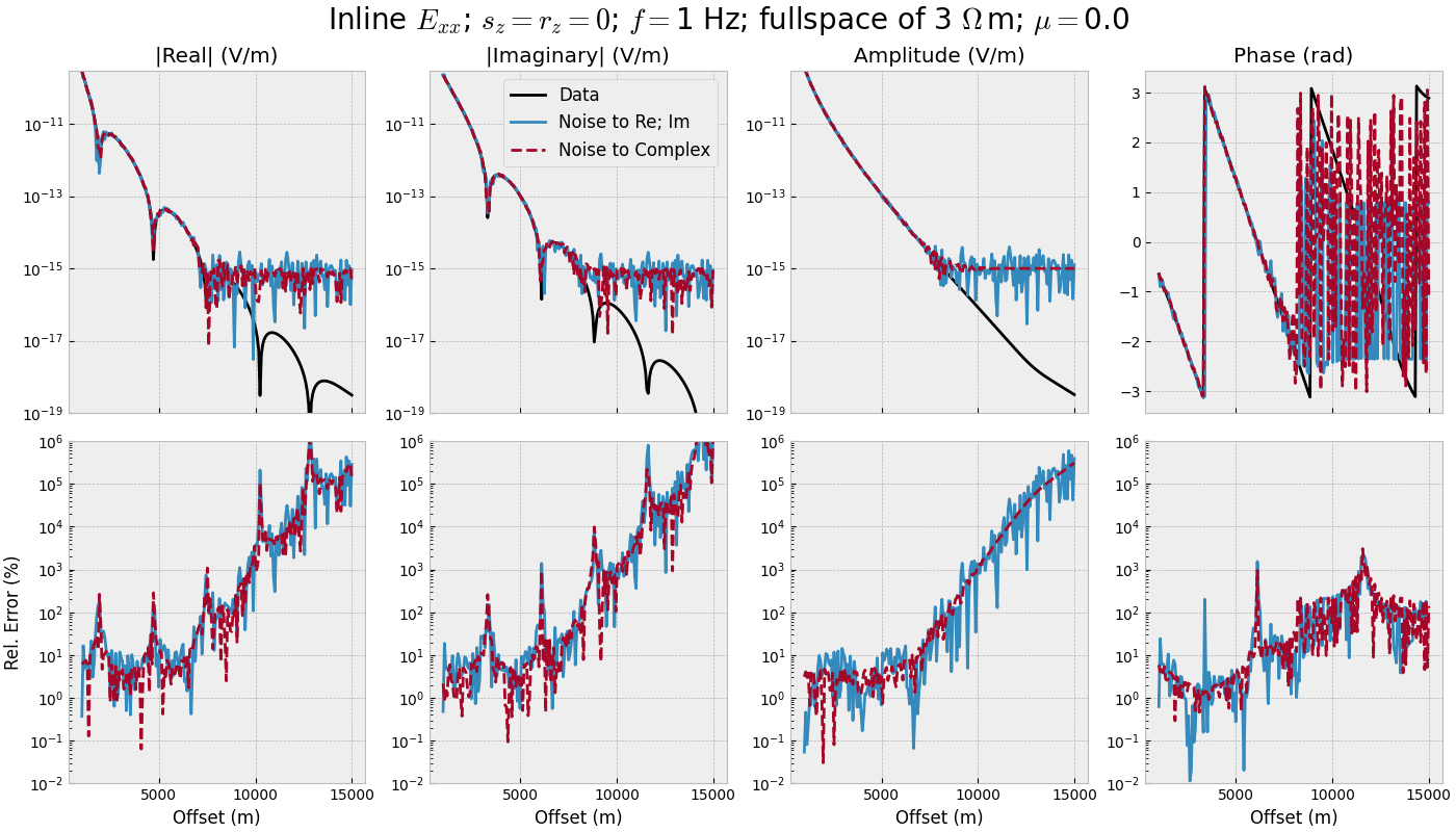
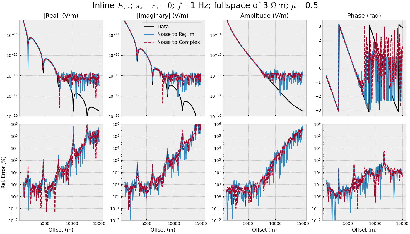
3.1 Offset-range for single frequency#
def offset_single(mu):
    """Single frequency, many offsets, one realization."""
    # Add noise
    inp = {'rel_error': rel_error, 'noise_floor': noise_floor, 'mu': mu}
    onoise_reim = add_noise(oresp, 'gaussian_correlated', **inp)
    onoise_comp = add_noise(oresp, 'white_noise', **inp)

    fig, axs = figure(offs, oresp, onoise_reim, onoise_comp)
    fig.suptitle(f"Inline $E_{{xx}}$; $s_z=r_z=0$; $f=${freq} Hz; "
                 f"fullspace of {model['res']} $\\Omega\\,$m; $\\mu=${mu}",
                 fontsize=20)

    for i in range(3):
        axs[0, i].set_ylim([1e-19, 3e-10])

    for i in range(4):
        axs[1, i].set_xlabel('Offset (m)')
        axs[1, i].set_yscale('log')
        axs[1, i].set_ylim([1e-2, 1e6])
offset_single(mu=0.0)
offset_single(mu=0.5)
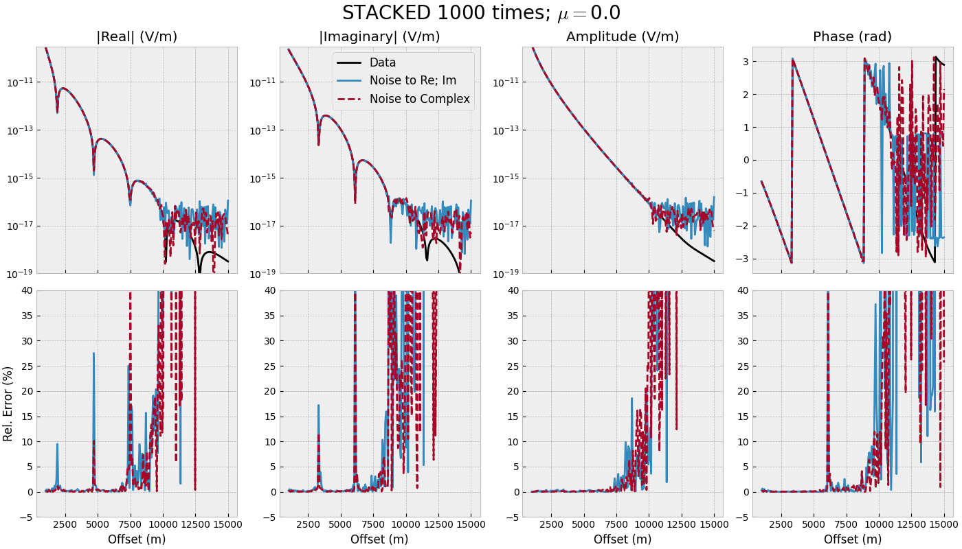
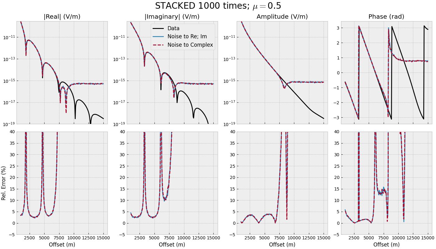
3.2 Offset-range for single frequency - STACKED#
def offset_stacked(mu):
    """Single frequency, many offsets, stacked."""
    # Stack noise
    inp = {'rel_error': rel_error, 'noise_floor': noise_floor, 'mu': mu}
    sonoise_reim = stack(n_stack, oresp, 'gaussian_correlated', **inp)
    sonoise_comp = stack(n_stack, oresp, 'white_noise', **inp)

    fig, axs = figure(offs, oresp, sonoise_reim, sonoise_comp)
    fig.suptitle(f"STACKED {n_stack} times; $\\mu=${mu}", fontsize=20)

    for i in range(3):
        axs[0, i].set_ylim([1e-19, 3e-10])

    for i in range(4):
        axs[1, i].set_xlabel('Offset (m)')
        axs[1, i].set_ylim([-5, 40])
offset_stacked(mu=0.0)
offset_stacked(mu=0.5)
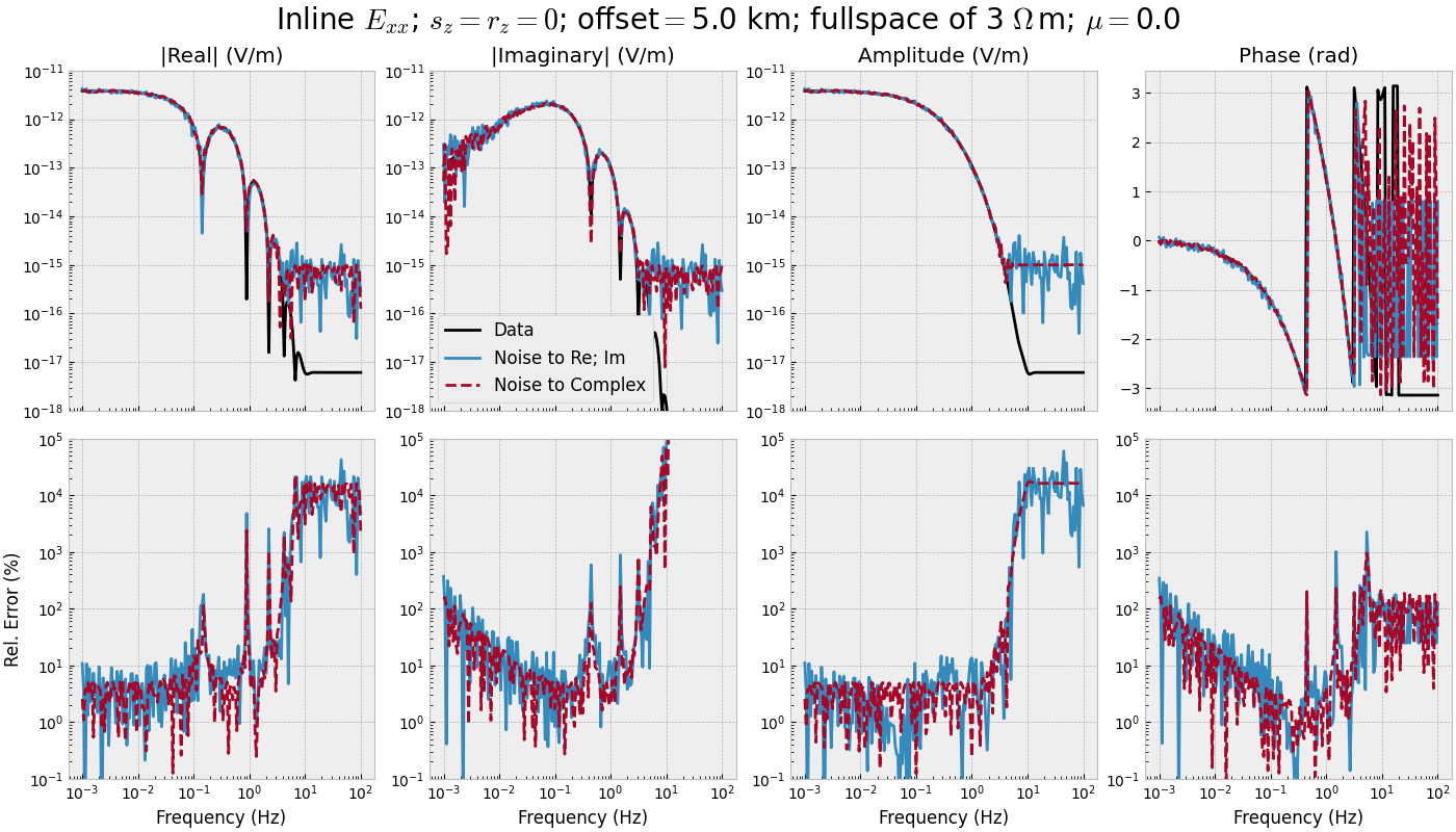
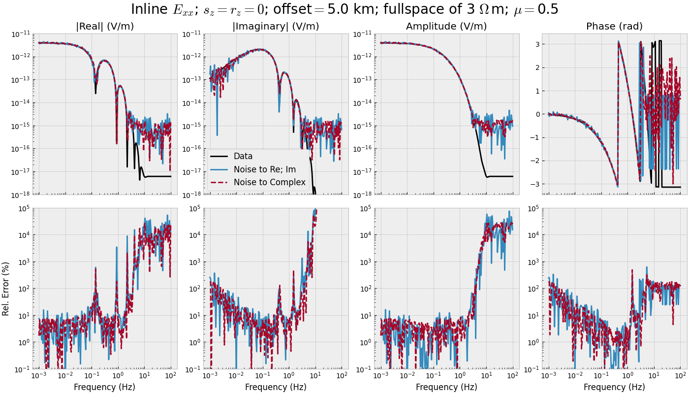
3.3 Frequency-range for single offset#
def frequency_single(mu):
    """Single offset, many frequencies, one realization."""
    # Add noise
    inp = {'rel_error': rel_error, 'noise_floor': noise_floor, 'mu': mu}
    fnoise_reim = add_noise(fresp, 'gaussian_correlated', **inp)
    fnoise_comp = add_noise(fresp, 'white_noise', **inp)

    fig, axs = figure(freqs, fresp, fnoise_reim, fnoise_comp)
    fig.suptitle(f"Inline $E_{{xx}}$; $s_z=r_z=0$; offset$=${off/1e3} km; "
                 f"fullspace of {model['res']} $\\Omega\\,$m; $\\mu=${mu}",
                 fontsize=20)

    for i in range(3):
        axs[0, i].set_ylim([1e-18, 1e-11])

    for i in range(4):
        axs[0, i].set_xscale('log')
        axs[1, i].set_xlabel('Frequency (Hz)')
        axs[1, i].set_yscale('log')
        axs[1, i].set_ylim([1e-1, 1e5])
frequency_single(mu=0.0)
frequency_single(mu=0.5)
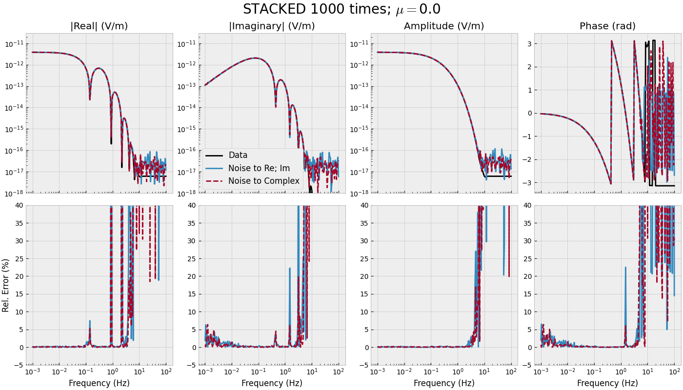
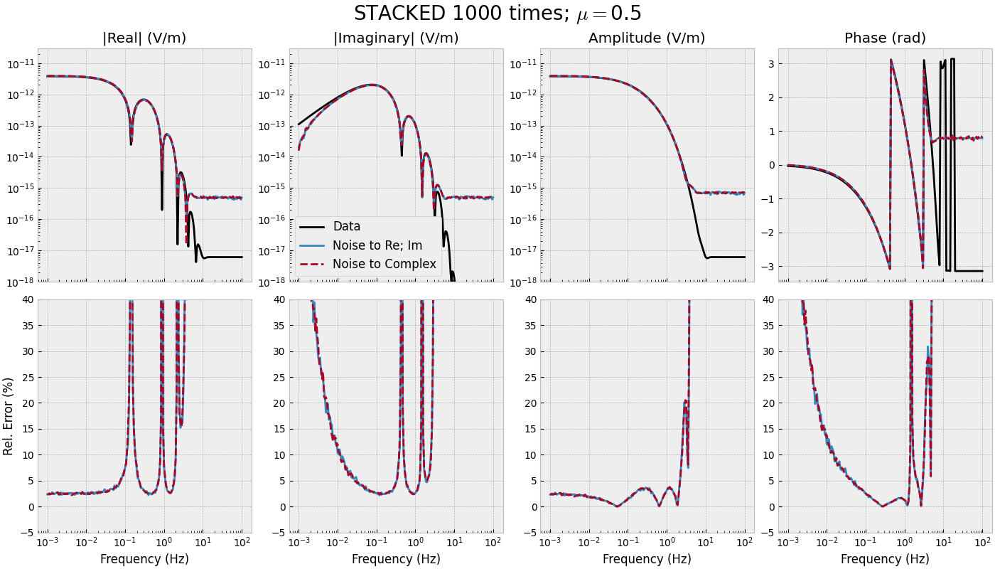
3.4 Frequency-range for single offset - STACKED#
def frequency_stacked(mu):
    """Single offset, many frequencies, stacked."""
    # Stack noise
    inp = {'rel_error': rel_error, 'noise_floor': noise_floor, 'mu': mu}
    sfnoise_reim = stack(n_stack, fresp, 'gaussian_correlated', **inp)
    sfnoise_comp = stack(n_stack, fresp, 'white_noise', **inp)

    fig, axs = figure(freqs, fresp, sfnoise_reim, sfnoise_comp)
    fig.suptitle(f"STACKED {n_stack} times; $\\mu=${mu}", fontsize=20)

    for i in range(3):
        axs[0, i].set_ylim([1e-18, 3e-11])

    for i in range(4):
        axs[0, i].set_xscale('log')
        axs[1, i].set_xlabel('Frequency (Hz)')
        axs[1, i].set_ylim([-5, 40])
frequency_stacked(mu=0.0)
frequency_stacked(mu=0.5)
empymod.Report()
Total running time of the script: (0 minutes 19.098 seconds)
Estimated memory usage: 194 MB