Note
Go to the end to download the full example code.
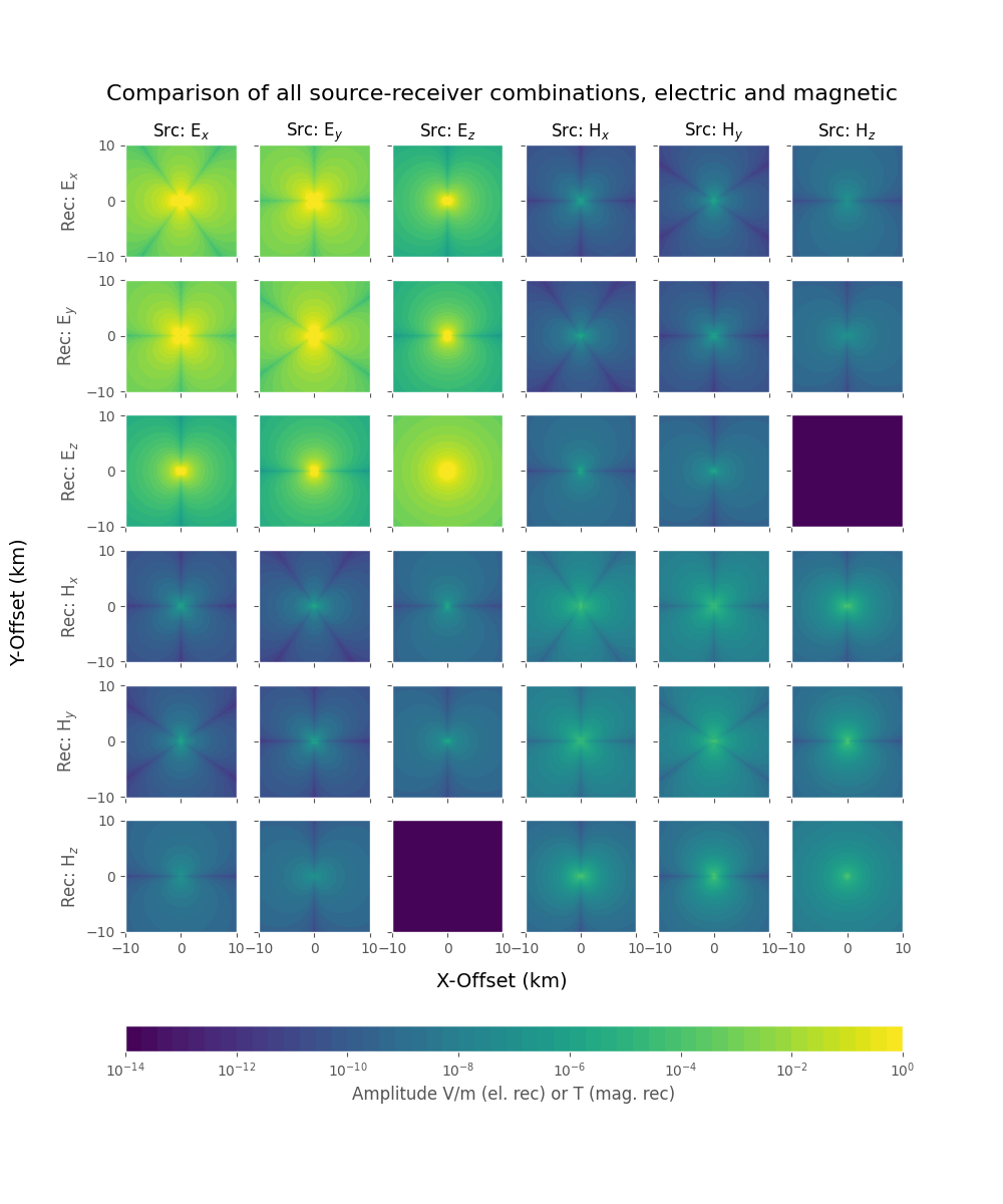
Comparison of all source-receiver combinations#
Comparison of all source-receiver combinations; both electric and magnetic.
We compute the secondary field for a simple model of a 1 Ωm halfspace below air. The source is 50 m above the surface in the air, receivers are on the surface, frequency is 1 Hz.
import empymod
import numpy as np
import matplotlib.pyplot as plt
plt.style.use('ggplot')
Define Model#
x = np.linspace(-10, 10, 101)*1000
rx = np.tile(x[:, None], x.size)
ry = rx.transpose()
inp = {
    'src': [0, 0, -50],
    'rec': [rx.ravel(), ry.ravel(), 0],
    'depth': 0,
    'res': [2e14, 1],
    'freqtime': 1,
    'xdirect': None,  # Secondary field comp., req. empymod >= v1.6.1.
    'htarg': {'pts_per_dec': -1},  # To speed-up the computation
    'verb': 0,
}
Compute#
[11 12 13 14 15 16 21 22 23 24 25 26 31 32 33 34 35 36 41 42 43 44 45 46
 51 52 53 54 55 56 61 62 63 64 65 66]
Plot#
fig, axs = plt.subplots(6, 6, figsize=(10, 11.5), constrained_layout=True)
axs = axs.ravel()
fig.suptitle('Comparison of all source-receiver combinations, electric ' +
             'and magnetic', fontsize=16)

# Labels
label1 = ['ˣ', 'ʸ', 'ᶻ']
label2 = ['E', 'H']

# Colour settings
vmin = 1e-14
vmax = 1e-0
props = {'levels': np.logspace(np.log10(vmin), np.log10(vmax), 50),
         'locator': plt.matplotlib.ticker.LogLocator()}

# Loop over combinations
for i, val in enumerate(pab):
    ax = axs[i]

    # Axis settings
    ax.set_xlim(min(x)/1000, max(x)/1000)
    ax.set_ylim(min(x)/1000, max(x)/1000)
    ax.axis('equal')

    # Plot the contour
    cf = ax.contourf(rx/1000, ry/1000, fs[str(val)].clip(vmin, vmax), **props)

    # Add titels
    if i < 6:
        label = 'Src: '
        label += label2[0] if i < 3 else label2[1]
        label += label1[i % 3]
        ax.xaxis.set_label_position("top")
        ax.set_xlabel(label, fontsize=12)
    if i % 6 == 5:
        label = 'Rec: '
        label += label2[0] if i < 18 else label2[1]
        label += label1[(i // 6) % 3]
        ax.yaxis.set_label_position("right")
        ax.set_ylabel(label, fontsize=12)

    # Remove unnecessary tick labels
    if i < 30:
        ax.set_xticks([-10, 0, 10], ())
    if i % 6 != 0:
        ax.set_yticks([-10, 0, 10], ())

    # Add offset labels
    if i == 32:
        ax.set_xlabel('X-Offset (km)', fontsize=14)
    elif i == 18:
        ax.set_ylabel('y-Offset (km)', fontsize=14)

# Colour bar
cb = plt.colorbar(
        cf, ax=axs, orientation='horizontal',
        ticks=np.logspace(np.log10(vmin), np.log10(vmax), 8))
cb.set_label('Amplitude in V/m (electric receiver) or T (magnetic receiver)')
empymod.Report()
Total running time of the script: (0 minutes 2.896 seconds)
Estimated memory usage: 217 MB