Improve land CSEM calculation

The problem

There exists a numerical singularity in the wavenumber-frequency domain. This singularity is always present, but it is usually neglectible except when the resistivity is very high (like air; hence conductivity goes to zero and therefore the real part of \(\eta_H\), \(\eta_V\) goes to zero) and source and receiver are close to this boundary. So unfortunately exactly in the case of a land CSEM survey.

This singularity leads to noise at very high frequencies and therefore at very early times because the Hankel transform cannot handle the singularity correctly (or, if you would choose a sufficiently precise quadrature, it would take literally forever to calculate it).

The “solution”

Electric permittivity (\(\varepsilon_H\), \(\varepsilon_V\)) are set to 1 by default. They are not important for the frequency range of CSEM. By setting the electric permittivity of the air-layer to 0, the singularity disapears, which subsquently improves a lot the time-domain result for land CSEM. It therefore uses the diffusive approximation for the air layer, but again, that doesn’t matter for the frequencies required for CSEM.

import empymod
import numpy as np
import matplotlib.pyplot as plt
plt.style.use('ggplot')

Define model

# Times (s)
t = np.logspace(-2, 1, 301)

# Model
model = {
    'src': [0, 0, 0.001],           # Src at origin, slightly below interface
    'rec': [6000, 0, 0.0001],       # 6 km off., in-line, slightly bel. interf.
    'depth': [0, 2000, 2100],       # Target of 100 m at 2 km depth
    'res': [2e14, 10, 100, 10],     # Res: [air, overb., target, half-space]
    'epermH': [1, 1, 1, 1],         # epermH/epermV: correspond to the default
    'epermV': [1, 1, 1, 1],         # #              values if not provided
    'freqtime': t,                  # Times
    'signal': 0,                    # 0: Impulse response
    'ftarg': 'key_81_CosSin_2009',  # Choose a shorter filter then the default
    'verb': 1,                      # Verbosity; set to 3 to see all parameters
}

Calculate

# Calculate with default eperm_air = 1
res_1 = empymod.dipole(**model)

# Set horizontal and vertical electric permittivity of air to 0
model['epermH'][0] = 0
model['epermV'][0] = 0

# Calculate with eperm_air = 0
res_0 = empymod.dipole(**model)

Plot result

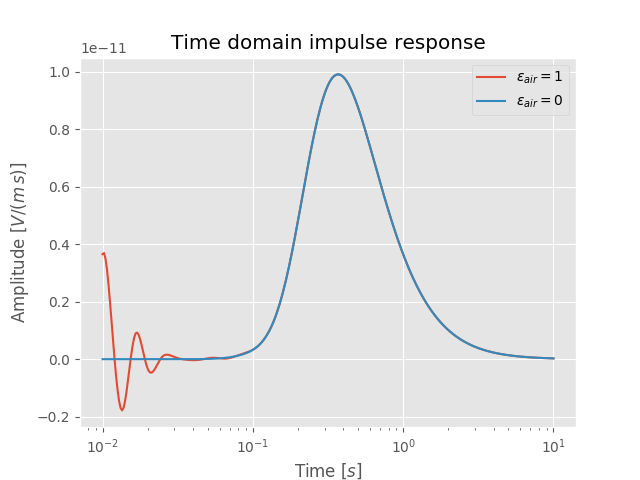
As it can be seen, setting \(\varepsilon_{air} =\) 0 improves the land CSEM result significantly for earlier times, where the signal should be zero.

plt.figure()

plt.title('Time domain impulse response')
plt.semilogx(t, res_1, label=r'$\varepsilon_{air}=1$')
plt.semilogx(t, res_0, label=r'$\varepsilon_{air}=0$')
plt.xlabel(r'Time $[s]$')
plt.ylabel(r'Amplitude $[V/(m\,s)]$')
plt.legend()

plt.show()

Version 1.7.0 and older

If you use a version of empymod that is smaller than 1.7.1 and set \(\varepsilon_H\), \(\varepsilon_V\) to zero you will see the following warning,

* WARNING :: Parameter epermH < 1e-20  are set to 1e-20 !
* WARNING :: Parameter epermV < 1e-20  are set to 1e-20 !

and the values will be re-set to the defined minimum value, which is by default 1e-20. Using a value of 1e-20 for epermH/epermV is also working just fine for land CSEM.

It is possible to change the minimum to zero for these old versions of empymod. However, there is a caveat: In empymod v1.7.0 and older, the min_param-parameter also checks frequency and anisotropy. If you set min_param=0, and provide empymod with resistivities or anisotropies equals to zero, empymod will crash due to division by zero errors (avoiding division by zero is the purpose behind the min_param-parameter).

To change the min_param-parameter do:

import empymod
empymod.set_minimum(min_param=0)

empymod.Report()

Estimated memory usage: 8 MB