Note
Click here to download the full example code
Cole-Cole
There are various different definitions of a Cole-Cole model, see for instance Tarasov and Titov (2013). We try a few different ones here, but you can supply your preferred version.
The original Cole-Cole (1940) model was formulated for the complex dielectric permittivity. It is reformulated to conductivity to use it for IP,
Another, similar model is given by Pelton et al. (1978),
Equation (2) is just like equation (1), but replaces \(\sigma\) by \(\rho\). However, mathematically they are not the same. Substituting \(\rho = 1/\sigma\) in the latter and resolving it for \(\sigma\) will not yield the former. Equation (2) is usually written in the following form, using the chargeability \(m = (\rho_0-\rho_\infty)/\rho_0\),
In all cases we add the part coming from the dielectric permittivity (displacement currents), even tough it usually doesn’t matter in the frequency range of IP.
References
- Cole, K.S., and R.H. Cole, 1941, Dispersion and adsorption in dielectrics. I. Alternating current characteristics; Journal of Chemical Physics, Volume 9, Pages 341-351, doi: [10.1063/1.1750906](https://doi.org/10.1063/1.1750906).
- Pelton, W.H., S.H. Ward, P.G. Hallof, W.R. Sill, and P.H. Nelson, 1978, Mineral discrimination and removal of inductive coupling with multifrequency IP, Geophysics, Volume 43, Pages 588-609, doi: [10.1190/1.1440839](https://doi.org/10.1190/1.1440839).
- Tarasov, A., and K. Titov, 2013, On the use of the Cole–Cole equations in spectral induced polarization; Geophysical Journal International, Volume 195, Issue 1, Pages 352-356, doi: [10.1093/gji/ggt251](https://doi.org/10.1093/gji/ggt251).
import empymod
import numpy as np
import matplotlib.pyplot as plt
plt.style.use('ggplot')
Use empymod with user-def. func. to adjust \(\eta\) and \(\zeta\)
In principal it is always best to write your own modelling routine if you
want to adjust something. Just copy empymod.dipole or empymod.bipole
as a template, and modify it to your needs. Since empymod v1.7.4,
however, there is a hook which allows you to modify \(\eta_h, \eta_v,
\zeta_h\), and \(\zeta_v\) quite easily.
The trick is to provide a dictionary (we name it inp here) instead of the
resistivity vector in res. This dictionary, inp, has two mandatory
plus optional entries: - res: the resistivity vector you would have
provided normally (mandatory).
- A function name, which has to be either or both of (mandatory):
func_eta: To adjustetaHandetaV, orfunc_zeta: to adjustzetaHandzetaV.
- In addition, you have to provide all parameters you use in
func_eta/func_zetaand are not already provided toempymod. All additional parameters must have #layers elements.
The functions func_eta and func_zeta must have the following
characteristics:
- The signature is
func(inp, p_dict), whereinpis the dictionary you provide, andp_dictis a dictionary that contains all parameters so far calculated in empymod [locals()].
- It must return
etaH, etaViffunc_eta, orzetaH, zetaViffunc_zeta.
Dummy example
def my_new_eta(inp, p_dict):
    # Your calculations, using the parameters you provided
    # in ``inp`` and the parameters from empymod in ``p_dict``.
    # In the example below, we provide, e.g., inp['tau']
    return etaH, etaV
And then you call empymod with res = {'res': res-array, 'tau': tau,
'func_eta': my_new_eta}.
Define the Cole-Cole model
In this notebook we exploit this hook in empymod to calculate \(\eta_h\) and \(\eta_v\) with the Cole-Cole model. By default, \(\eta_h\) and \(\eta_v\) are calculated like this:
With this function we recalculate it. We replace the real part, the resistivity \(\rho\), in equations (4) and (5) by the complex, frequency-dependent Cole-Cole resistivity [\(\rho(\omega)\)], as given, for instance, in equations (1)-(3). Then we add back the imaginary part coming from thet dielectric permittivity (basically zero for low frequencies).
Note that in this notebook we use this hook to model relaxation in the low frequency spectrum for IP measurements, replacing \(\rho\) by a frequency-dependent model \(\rho(\omega)\). However, this could also be used to model dielectric phenomena in the high frequency spectrum, replacing \(\varepsilon_r\) by a frequency-dependent formula \(\varepsilon_r(\omega)\).
def cole_cole(inp, p_dict):
    """Cole and Cole (1941)."""

    # Calculate complex conductivity from Cole-Cole
    iotc = np.outer(2j*np.pi*p_dict['freq'], inp['tau'])**inp['c']
    condH = inp['cond_8'] + (inp['cond_0']-inp['cond_8'])/(1+iotc)
    condV = condH/p_dict['aniso']**2

    # Add electric permittivity contribution
    etaH = condH + 1j*p_dict['etaH'].imag
    etaV = condV + 1j*p_dict['etaV'].imag

    return etaH, etaV


def pelton_et_al(inp, p_dict):
    """ Pelton et al. (1978)."""

    # Calculate complex resistivity from Pelton et al.
    iotc = np.outer(2j*np.pi*p_dict['freq'], inp['tau'])**inp['c']
    rhoH = inp['rho_0']*(1 - inp['m']*(1 - 1/(1 + iotc)))
    rhoV = rhoH*p_dict['aniso']**2

    # Add electric permittivity contribution
    etaH = 1/rhoH + 1j*p_dict['etaH'].imag
    etaV = 1/rhoV + 1j*p_dict['etaV'].imag

    return etaH, etaV
Example
Two half-space model, air above earth:
x-directed sourcer at the surface
x-directed receiver, also at the surface, inline at an offset of 500 m.
Switch-on time-domain response
Isotropic
Model [air, subsurface]
- \(\rho_\infty = 1/\sigma_\infty =\) [2e14, 10]
- \(\rho_0 = 1/\sigma_0 =\) [2e14, 5]
- \(\tau =\) [0, 1]
- \(c =\) [0, 0.5]
# Times
times = np.logspace(-2, 2, 101)
# Model parameter which apply for all
model = {
'src': [0, 0, 1e-5, 0, 0],
'rec': [500, 0, 1e-5, 0, 0],
'depth': 0,
'freqtime': times,
'signal': 1,
'verb': 1
}
# Collect Cole-Cole models
res_0 = np.array([2e14, 10])
res_8 = np.array([2e14, 5])
tau = [0, 1]
c = [0, 0.5]
m = (res_0-res_8)/res_0
cole_model = {'res': res_0, 'cond_0': 1/res_0, 'cond_8': 1/res_8,
'tau': tau, 'c': c, 'func_eta': cole_cole}
pelton_model = {'res': res_0, 'rho_0': res_0, 'm': m,
'tau': tau, 'c': c, 'func_eta': pelton_et_al}
# Calculate
out_bipole = empymod.bipole(res=res_0, **model)
out_cole = empymod.bipole(res=cole_model, **model)
out_pelton = empymod.bipole(res=pelton_model, **model)
# Plot
plt.figure()
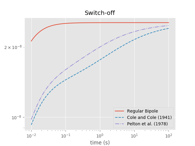
plt.title('Switch-off')
plt.plot(times, out_bipole, label='Regular Bipole')
plt.plot(times, out_cole, '--', label='Cole and Cole (1941)')
plt.plot(times, out_pelton, '-.', label='Pelton et al. (1978)')
plt.legend()
plt.yscale('log')
plt.xscale('log')
plt.xlabel('time (s)')
plt.show()
empymod.Report()
Total running time of the script: ( 0 minutes 1.215 seconds)
Estimated memory usage: 11 MB