Hunziker et al., 2015, Geophysics

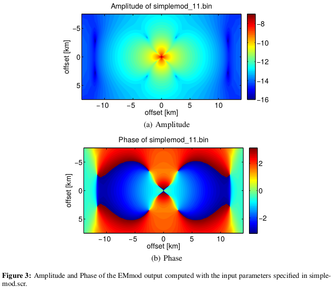
Reproducing Figure 3 of the manual from EMmod. This example does, as such, not actually reproduce a figure of Hunziker et al., 2015, but of the manual that comes with the software accompanying the paper. With the software comes an example input file named simplemod.scr, and the corresponding result is shown in the manual of the code in Figure 3.

If you are interested in reproducing the figures of the actual paper have a look at the notebooks in the repo article-geo2017.

Reference

• Hunziker, J., J. Thorbecke, and E. Slob, 2015, The electromagnetic response in a layered vertical transverse isotropic medium: A new look at an old problem: Geophysics, 80(1), F1–F18; DOI: 10.1190/geo2013-0411.1; Software: software.seg.org/2015/0001.

import empymod
import numpy as np
import matplotlib.pyplot as plt

Compute the data

Compute the electric field with the parameters defined in simplemod.scr.

# x- and y-offsets
x = np.arange(4000)*7-1999.5*7
y = np.arange(1500)*10-749.5*10

# Create 2D arrays of them
rx = np.repeat([x, ], np.size(y), axis=0)
ry = np.repeat([y, ], np.size(x), axis=0)
ry = ry.transpose()

# Compute the electric field
efield = empymod.dipole(
    src=[0, 0, 150],
    rec=[rx.ravel(), ry.ravel(), 200],
    depth=[0, 200, 1000, 1200],
    res=[2e14, 1/3, 1, 50, 1],
    aniso=[1, 1, np.sqrt(10), 1, 1],
    freqtime=0.5,
    epermH=[1, 80, 17, 2.1, 17],
    epermV=[1, 80, 17, 2.1, 17],
    mpermH=[1, 1, 1, 1, 1],
    mpermV=[1, 1, 1, 1, 1],
    ab=11,
    htarg={'pts_per_dec': -1},
).reshape(np.shape(rx))

Out:

:: empymod END; runtime = 0:00:02.381813 :: 1 kernel call(s)

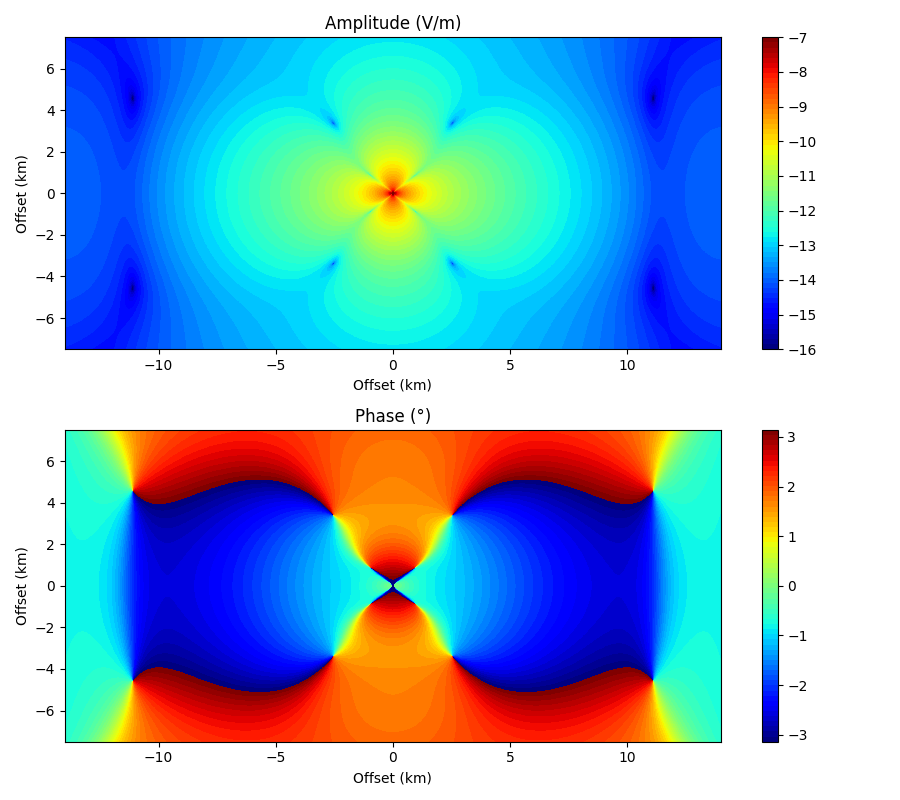
Plot

# Create a similar colormap as Hunziker et al., 2015.
cmap = plt.cm.get_cmap("jet", 61)

plt.figure(figsize=(9, 8))

# 1. Amplitude
plt.subplot(211)
plt.title('Amplitude (V/m)')
plt.xlabel('Offset (km)')
plt.ylabel('Offset (km)')
plt.pcolormesh(x/1e3, y/1e3, np.log10(efield.amp()),
               cmap=cmap, vmin=-16, vmax=-7, shading='nearest')
plt.colorbar()

# 2. Phase
plt.subplot(212)
plt.title('Phase (°)')
plt.xlabel('Offset (km)')
plt.ylabel('Offset (km)')
plt.pcolormesh(x/1e3, y/1e3, efield.pha(deg=False, unwrap=False, lag=True),
               cmap=cmap, vmin=-np.pi, vmax=np.pi, shading='nearest')
plt.colorbar()

plt.tight_layout()
plt.show()

Original Figure

Figure 3 of the manual of EMmod.

empymod.Report()

Sun Jul 04 11:00:10 2021 UTC
OS	Linux	CPU(s)	2	Machine	x86_64
Architecture	64bit	RAM	7.5 GiB	Environment	Python
Python 3.8.6 (default, Oct 19 2020, 15:10:29) [GCC 7.5.0]
numpy	1.21.0	scipy	1.7.0	numba	0.53.1
empymod	2.1.2	IPython	7.25.0	matplotlib	3.4.2

Estimated memory usage: 836 MB

Constable and Weiss, 2006 Ward and Hohmann, 1988, SEG