Note
Click here to download the full example code
DC apparent resistivity
DC apparent resistivity, dipole-dipole configuration.
There are various DC sounding layouts, the most common ones being Schlumberger, Wenner, pole-pole, pole-dipole, and dipole-dipole, at which we have a look here.
Dipole-dipole layout as shown in figure 8.32 in Kearey et al. (2002):
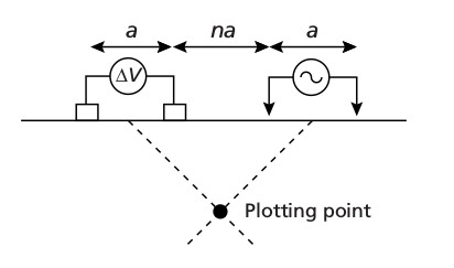
The apparent resistivity \(\rho_a\) of the plotting point is then computed with
where \(V\) is measured Voltage, \(I\) is source strength, \(a\) is dipole length, and \(n\) is the factor of source-receiver separation.
References
Kearey, P., M. Brooks, and I. Hill, 2002, An introduction to geophysical exploration, 3rd ed.: Blackwell Scientific Publications, ISBN: 0 632 04929 4.
import empymod
import numpy as np
import matplotlib.pyplot as plt
plt.style.use('ggplot')
Compute \(\boldsymbol{\rho_a}\)
First we define a function to compute apparent resistivity for a given model and given source and receivers.
def comp_appres(depth, res, a, n, srcpts=1, recpts=1, verb=1):
    """Return apparent resistivity for dipole-dipole DC measurement

        rho_a = V/I pi a n (n+1) (n+2).

    Returns die apparent resistivity due to:
    - Electric source, inline (y = 0 m).
    - Source of 1 A strength.
    - Source and receiver are located at the air-interface.
    - Source is centered at x = 0 m.

    Note: DC response can be obtained by either t->infinity s or f->0 Hz. f = 0
          Hz is much faster, as there is no Fourier transform involved and only
          a single frequency has to be computed. By default, the minimum
          frequency in empymod is 1e-20 Hz. The difference between the signals
          for 1e-20 Hz and 0 Hz is very small.

    For more explanation regarding input parameters see `empymod.model`.

    Parameters
    ----------
    depth : Absolute depths of layer interfaces, without air-interface.
    res : Resistivities of the layers, one more than depths (lower HS).
    a : Dipole length.
    n : Separation factors.
    srcpts, recpts : If < 3, bipoles are approximated as dipoles.
    verb : Verbosity.

    Returns
    -------
    rho_a : Apparent resistivity.
    AB2 : Src/rec-midpoints

    """

    # Get offsets between src-midpoint and rec-midpoint, AB
    AB = (n+1)*a

    # Collect model, putting source and receiver slightly (1e-3 m) into the
    # ground.
    model = {
        'src': [-a/2, a/2, 0, 0, 1e-3, 1e-3],
        'rec': [AB-a/2, AB+a/2, AB*0, AB*0, 1e-3, 1e-3],
        'depth': np.r_[0, np.array(depth, ndmin=1)],
        'freqtime': 1e-20,  # Smaller f would be set to 1e-20 be empymod.
        'verb': verb,       # Setting it to 1e-20 avoids warning-message.
        'res': np.r_[2e14, np.array(res, ndmin=1)],
        'strength': 1,      # So it is NOT normalized to 1 m src/rec.
        'htarg': {'pts_per_dec': -1},
    }

    return np.real(empymod.bipole(**model))*np.pi*a*n*(n+1)*(n+2), AB/2
Plot-function
Second we create a plot-function, which includes the call to comp_appres, to use for a couple of different models.
def plotit(depth, a, n, res1, res2, res3, title):
    """Call `comp_appres` and plot result."""

    # Compute the three different models
    rho1, AB2 = comp_appres(depth, res1, a, n)
    rho2, _ = comp_appres(depth, res2, a, n)
    rho3, _ = comp_appres(depth, res3, a, n)

    # Create figure
    plt.figure()

    # Plot curves
    plt.loglog(AB2, rho1, label='Case 1')
    plt.plot(AB2, rho2, label='Case 2')
    plt.plot(AB2, rho3, label='Case 3')

    # Legend, labels
    plt.legend(loc='best')
    plt.title(title)
    plt.xlabel('AB/2 (m)')
    plt.ylabel(r'Apparent resistivity $\rho_a (\Omega\,$m)')

    plt.show()
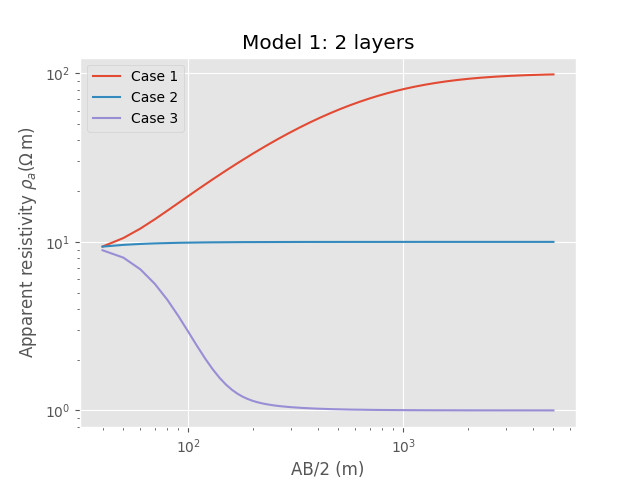
Model 1: 2 layers
layer |
depth (m) |
resistivity (Ohm m) |
|---|---|---|
air |
\(-\infty\) - 0 |
2e14 |
layer 1 |
0 - 50 |
10 |
layer 2 |
50 - \(\infty\) |
100 / 10 / 1 |
plotit(
    50,                 # Depth
    20,                 # a (src- and rec-lengths)
    np.arange(3, 500),  # n
    [10, 100],          # Case 1
    [10,  10],          # Case 2
    [10,   1],          # Case 3
    'Model 1: 2 layers')
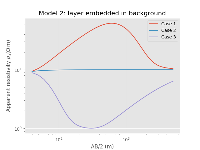
Model 2: layer embedded in background
layer |
depth (m) |
resistivity (Ohm m) |
|---|---|---|
air |
\(-\infty\) - 0 |
2e14 |
layer 1 |
0 - 50 |
10 |
layer 2 |
50 - 500 |
100 / 10 / 1 |
layer 3 |
500 - \(\infty\) |
10 |
plotit(
    [50, 500],          # Depth
    20,                 # a (src- and rec-lengths)
    np.arange(3, 500),  # n
    [10, 100, 10],      # Case 1
    [10,  10, 10],      # Case 2
    [10,   1, 10],      # Case 3
    'Model 2: layer embedded in background')
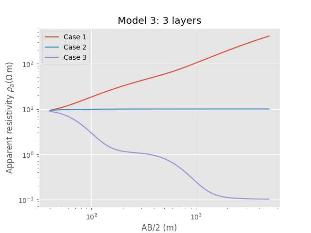
Model 3: 3 layers
layer |
depth (m) |
resistivity (Ohm m) |
|
|---|---|---|---|
air |
\(-\infty\) - 0 |
2e14 |
|
layer 1 |
0 - 50 |
10 |
|
layer 2 |
50 - 500 |
100 / 10 / 1 |
|
layer 3 |
500 - \(\infty\) | 1000 / 10 / 0.1 |
||
plotit(
    [50, 500],          # Depth
    20,                 # a (src- and rec-lengths)
    np.arange(3, 500),  # n
    [10, 100, 1000],    # Case 1
    [10,  10,   10],    # Case 2
    [10,   1,    0.1],  # Case 3
    'Model 3: 3 layers')
empymod.Report()
Total running time of the script: ( 0 minutes 2.004 seconds)
Estimated memory usage: 11 MB