Note
Click here to download the full example code
Ward and Hohmann, 1988, SEG
Frequency and time-domain modelling of magnetic loop sources and magnetic receivers.
Reproducing Figures 2.2-2.5, 4.2-4.5, and 4.7-4.8 of Ward and Hohmann (1988): Frequency- and time-domain isotropic solutions for a full-space (2.2-2.5) and a half-space (4.2-4.5, 4.7-4.8), where source and receiver are at the interface. Source is a loop, receiver is a magnetic dipole.
Reference
Ward, S. H., and G. W. Hohmann, 1988, Electromagnetic theory for geophysical applications, Chapter 4 of Electromagnetic Methods in Applied Geophysics: SEG, Investigations in Geophysics No. 3, 130–311; DOI: 10.1190/1.9781560802631.ch4.
import empymod
import numpy as np
from scipy.special import erf
import matplotlib.pyplot as plt
from scipy.constants import mu_0
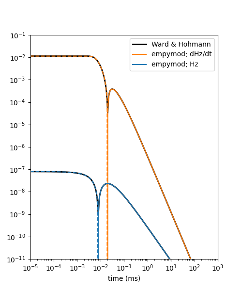
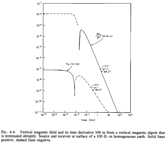
Ward and Hohmann, 1988, Fig 4.4
Ward and Hohmann (1988), Equations 4.69a and 4.70:
and
where
\(t\) is time in s, \(\rho\) is resistivity in \(\Omega\,\text{m}\), \(r\) is offset in m, and \(m\) the magnetic moment in \(\text{A}\,\text{m}^2\) .
Analytical solutions
def hz(t, res, r, m=1.):
    r"""Return equation 4.69a, Ward and Hohmann, 1988.

    Switch-off response (i.e., Hz(t)) of a homogeneous isotropic half-space,
    where the vertical magnetic source and receiver are at the interface.

    Parameters
    ----------
    t : array
        Times (t)
    res : float
        Halfspace resistivity (Ohm.m)
    r : float
        Offset (m)
    m : float, optional
        Magnetic moment, default is 1.

    Returns
    -------
    hz : array
        Vertical magnetic field (A/m)

    """
    theta = np.sqrt(mu_0/(4*res*t))
    theta_r = theta*r

    s = -(9/theta_r+4*theta_r)*np.exp(-theta_r**2)/np.sqrt(np.pi)
    s += erf(theta_r)*(9/(2*theta_r**2)-1)
    s *= m/(4*np.pi*r**3)

    return s
def dhzdt(t, res, r, m=1.):
    r"""Return equation 4.70, Ward and Hohmann, 1988.

    Impulse response (i.e., dHz(t)/dt) of a homogeneous isotropic half-space,
    where the vertical magnetic source and receiver are at the interface.

    Parameters
    ----------
    t : array
        Times (t)
    res : float
        Halfspace resistivity (Ohm.m)
    r : float
        Offset (m)
    m : float, optional
        Magnetic moment, default is 1.

    Returns
    -------
    dhz : array
        Time-derivative of the vertical magnetic field (A/m/s)

    """
    theta = np.sqrt(mu_0/(4*res*t))
    theta_r = theta*r

    s = (9 + 6 * theta_r**2 + 4 * theta_r**4) * np.exp(-theta_r**2)
    s *= -2 * theta_r / np.sqrt(np.pi)
    s += 9 * erf(theta_r)
    s *= -(m*res)/(2*np.pi*mu_0*r**5)

    return s
Survey parameters
time = np.logspace(-8, 0, 301)

src = [0, 0, 0, 0, 90]
rec = [100, 0, 0, 0, 90]
depth = 0
res = [2e14, 100]
Numerical result
eperm = [0, 0]  # Reduce early time numerical noise (diffusive approx for air)
inp = {'src': src, 'rec': rec, 'depth': depth, 'res': res,
       'freqtime': time, 'verb': 1, 'xdirect': True, 'epermH': eperm}

hz_num = empymod.loop(signal=-1, **inp)
dhz_num = empymod.loop(signal=0, **inp)
Plot the result
plt.figure(figsize=(5, 6))

plt.plot(time*1e3, abs(dhz_ana), 'k-', lw=2, label='Ward & Hohmann')
plt.plot(time*1e3, dhz_num, 'C1-', label='empymod; dHz/dt')
plt.plot(time*1e3, -dhz_num, 'C1--')

plt.plot(time*1e3, abs(hz_ana), 'k-', lw=2)
plt.plot(time*1e3, hz_num, 'C0-', label='empymod; Hz')
plt.plot(time*1e3, -hz_num, 'C0--')

plt.xscale('log')
plt.yscale('log')
plt.xlim([1e-5, 1e3])
plt.yticks(10**np.arange(-11., 0))
plt.ylim([1e-11, 1e-1])
plt.xlabel('time (ms)')
plt.legend()

plt.show()
Original Figure
The following examples are just compared to the figures, without the provided analytical solutions.
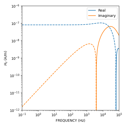
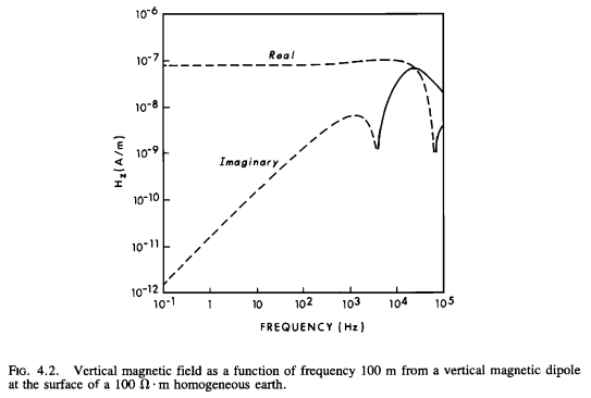
Ward and Hohmann, 1988, Fig 4.2
# Survey parameters
freq = np.logspace(-1, 5, 301)
src = [0, 0, 0, 0, 90]
rec = [100, 0, 0, 0, 90]
depth = 0
res = [2e14, 100]

# Computation
inp = {'src': src, 'rec': rec, 'depth': depth, 'res': res,
       'freqtime': freq, 'verb': 1}
fhz_num = empymod.loop(**inp)

# Figure
plt.figure(figsize=(5, 5))

plt.plot(freq, fhz_num.real, 'C0-', label='Real')
plt.plot(freq, -fhz_num.real, 'C0--')

plt.plot(freq, fhz_num.imag, 'C1-', label='Imaginary')
plt.plot(freq, -fhz_num.imag, 'C1--')

plt.xscale('log')
plt.yscale('log')
plt.xlim([1e-1, 1e5])
plt.ylim([1e-12, 1e-6])
plt.xlabel('FREQUENCY (Hz)')
plt.ylabel('$H_z$ (A/m)')
plt.legend()

plt.tight_layout()

plt.show()
Original Figure
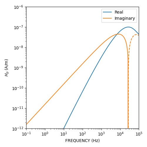
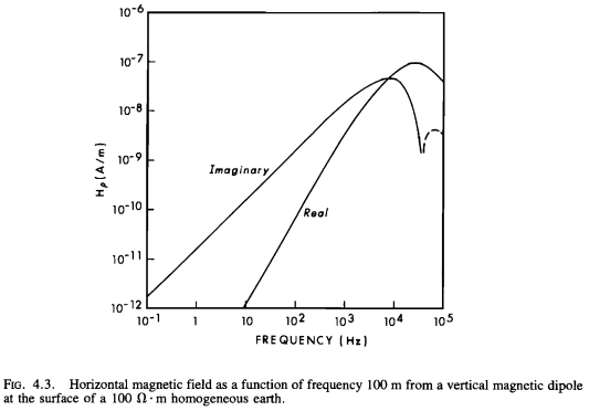
Ward and Hohmann, 1988, Fig 4.3
# Survey parameters
freq = np.logspace(-1, 5, 301)
src = [0, 0, 0, 0, 90]
rec = [100, 0, 0, 0, 0]
depth = 0
res = [2e14, 100]

# Computation
inp = {'src': src, 'rec': rec, 'depth': depth, 'res': res,
       'freqtime': freq, 'verb': 1}
fhz_num = empymod.loop(**inp)

# Figure
plt.figure(figsize=(5, 5))

plt.plot(freq, fhz_num.real, 'C0-', label='Real')
plt.plot(freq, -fhz_num.real, 'C0--')

plt.plot(freq, fhz_num.imag, 'C1-', label='Imaginary')
plt.plot(freq, -fhz_num.imag, 'C1--')

plt.xscale('log')
plt.yscale('log')
plt.xlim([1e-1, 1e5])
plt.ylim([1e-12, 1e-6])
plt.xlabel('FREQUENCY (Hz)')
plt.ylabel(r'$H_{\rho}$ (A/m)')
plt.legend()

plt.tight_layout()

plt.show()
Original Figure
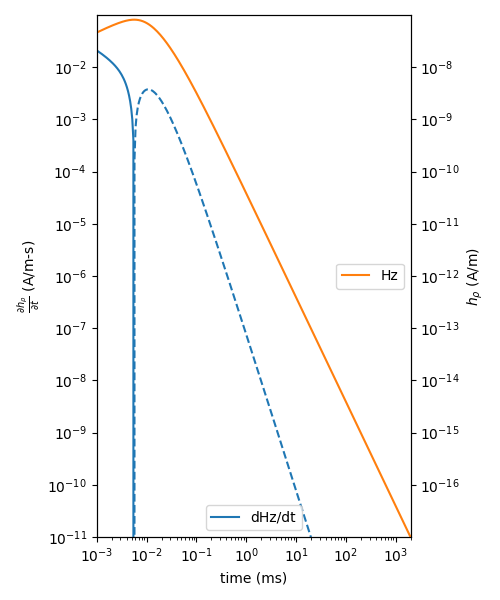
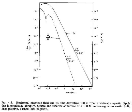
Ward and Hohmann, 1988, Fig 4.5
# Survey parameters
time = np.logspace(-6, 0.5, 301)
src = [0, 0, 0, 0, 90]
rec = [100, 0, 0, 0, 0]
depth = 0
res = [2e14, 100]

# Computation
inp = {'src': src, 'rec': rec, 'depth': depth, 'res': res,
       'epermH': eperm, 'freqtime': time, 'verb': 1}
fhz_num = empymod.loop(signal=1, **inp)
fdhz_num = empymod.loop(signal=0, **inp)

# Figure
plt.figure(figsize=(5, 6))

ax1 = plt.subplot(111)
plt.plot(time*1e3, fdhz_num, 'C0-', label='dHz/dt')
plt.plot(time*1e3, -fdhz_num, 'C0--')

plt.xscale('log')
plt.yscale('log')
plt.xlim([1e-3, 2e3])
plt.yticks(10**np.arange(-11., -1))
plt.ylim([1e-11, 1e-1])
plt.xlabel('time (ms)')
plt.ylabel(r'$\frac{\partial h_{\rho}}{\partial t}$ (A/m-s)')
plt.legend(loc=8)

ax2 = ax1.twinx()

plt.plot(time*1e3, fhz_num, 'C1-', label='Hz')
plt.plot(time*1e3, -fhz_num, 'C1--')

plt.xscale('log')
plt.yscale('log')
plt.xlim([1e-3, 2e3])
plt.yticks(10**np.arange(-16., -7))
plt.ylim([1e-17, 1e-7])
plt.ylabel(r'$h_{\rho}$ (A/m)')
plt.legend(loc=5)

plt.tight_layout()
plt.show()
Original Figure
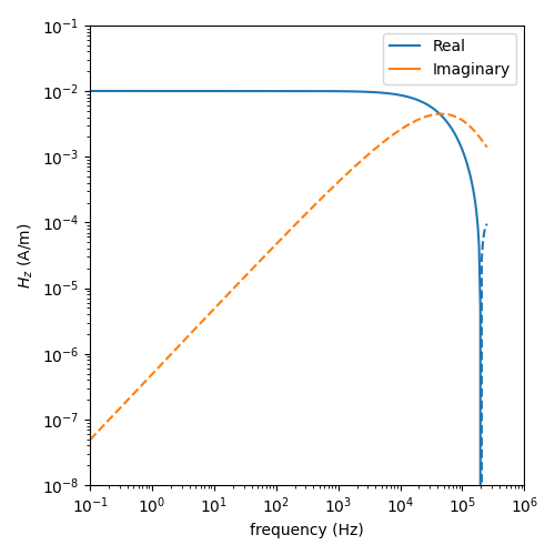
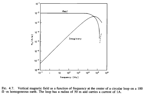
Ward and Hohmann, 1988, Fig 4.7
# Survey parameters
radius = 50
area = radius**2*np.pi
freq = np.logspace(-1, np.log10(250000), 301)
src = [radius, 0, 0, 90, 0]
rec = [0, 0, 0, 0, 90]
depth = 0
res = [2e14, 100]
strength = area/(radius/2)
mrec = True

# Computation
inp = {'src': src, 'rec': rec, 'depth': depth, 'res': res,
       'freqtime': freq, 'strength': strength, 'mrec': mrec,
       'verb': 1}
fhz_num = empymod.bipole(**inp)

# Figure
plt.figure(figsize=(5, 5))

plt.plot(freq, fhz_num.real, 'C0-', label='Real')
plt.plot(freq, -fhz_num.real, 'C0--')

plt.plot(freq, fhz_num.imag, 'C1-', label='Imaginary')
plt.plot(freq, -fhz_num.imag, 'C1--')

plt.xscale('log')
plt.yscale('log')
plt.xlim([1e-1, 1e6])
plt.ylim([1e-8, 1e-1])
plt.xlabel('frequency (Hz)')
plt.ylabel('$H_z$ (A/m)')
plt.legend()

plt.tight_layout()

plt.show()
Original Figure
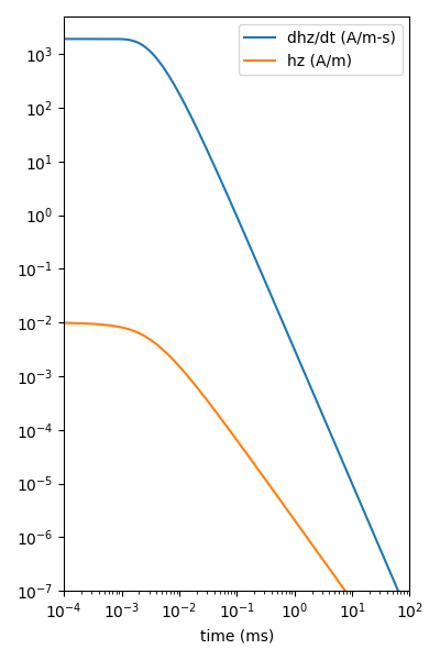
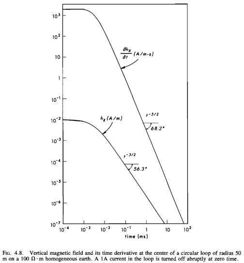
Ward and Hohmann, 1988, Fig 4.8
# Survey parameters
radius = 50
area = radius**2*np.pi
time = np.logspace(-7, -1, 301)
src = [radius, 0, 0, 90, 0]
rec = [0, 0, 0, 0, 90]
depth = 0
res = [2e14, 100]
strength = area/(radius/2)
mrec = True

# Computation
inp = {'src': src, 'rec': rec, 'depth': depth, 'res': res,
       'freqtime': time, 'strength': strength, 'mrec': mrec,
       'epermH': eperm, 'verb': 1}

fhz_num = empymod.bipole(signal=-1, **inp)
fdhz_num = empymod.bipole(signal=0, **inp)

# Figure
plt.figure(figsize=(4, 6))

ax1 = plt.subplot(111)
plt.plot(time*1e3, fdhz_num, 'C0-', label=r'dhz/dt (A/m-s)')
plt.plot(time*1e3, -fdhz_num, 'C0--')

plt.plot(time*1e3, fhz_num, 'C1-', label='hz (A/m)')
plt.plot(time*1e3, -fhz_num, 'C1--')

plt.xscale('log')
plt.yscale('log')
plt.xlim([1e-4, 1e2])
plt.yticks(10**np.arange(-7., 4))
plt.ylim([1e-7, 5e3])

plt.xlabel('time (ms)')
plt.legend()

plt.tight_layout()
plt.show()
Original Figure
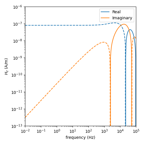
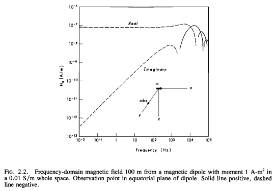
Ward and Hohmann, 1988, Fig 2.2
# Survey parameters
freq = np.logspace(-2, 5, 301)
src = [0, 0, 0, 0, 0]
rec = [0, 100, 0, 0, 0]
depth = []
res = 100

# Computation
inp = {'src': src, 'rec': rec, 'depth': depth, 'res': res,
       'freqtime': freq, 'verb': 1}
fhz_num = empymod.loop(**inp)

# Figure
plt.figure(figsize=(5, 5))

plt.plot(freq, fhz_num.real, 'C0-', label='Real')
plt.plot(freq, -fhz_num.real, 'C0--')

plt.plot(freq, fhz_num.imag, 'C1-', label='Imaginary')
plt.plot(freq, -fhz_num.imag, 'C1--')

plt.xscale('log')
plt.yscale('log')
plt.xlim([1e-2, 1e5])
plt.ylim([1e-13, 1e-6])
plt.xlabel('frequency (Hz)')
plt.ylabel('$H_z$ (A/m)')
plt.legend()

plt.tight_layout()

plt.show()
Original Figure
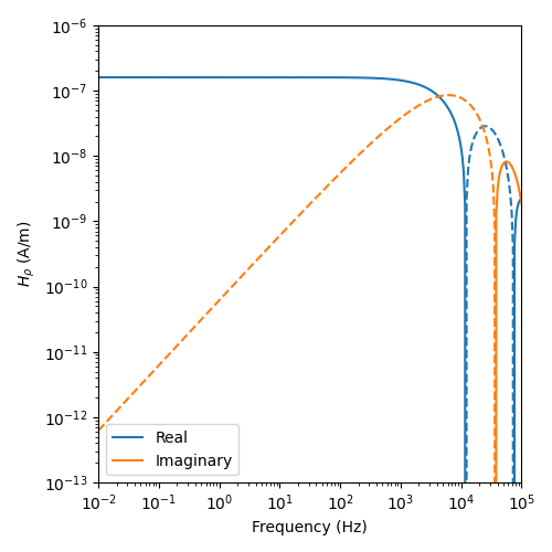
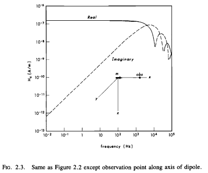
Ward and Hohmann, 1988, Fig 2.3
# Survey parameters
freq = np.logspace(-2, 5, 301)
src = [0, 0, 0, 0, 0]
rec = [100, 0, 0, 0, 0]
depth = []
res = 100

# Computation
inp = {'src': src, 'rec': rec, 'depth': depth, 'res': res,
       'freqtime': freq, 'verb': 1}
fhz_num = empymod.loop(**inp)

# Figure
plt.figure(figsize=(5, 5))

plt.plot(freq, fhz_num.real, 'C0-', label='Real')
plt.plot(freq, -fhz_num.real, 'C0--')

plt.plot(freq, fhz_num.imag, 'C1-', label='Imaginary')
plt.plot(freq, -fhz_num.imag, 'C1--')

plt.xscale('log')
plt.yscale('log')
plt.xlim([1e-2, 1e5])
plt.ylim([1e-13, 1e-6])
plt.xlabel('Frequency (Hz)')
plt.ylabel(r'$H_{\rho}$ (A/m)')
plt.legend()

plt.tight_layout()
plt.show()
Original Figure
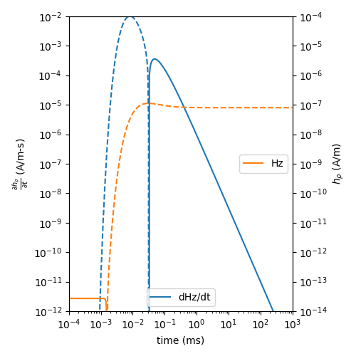
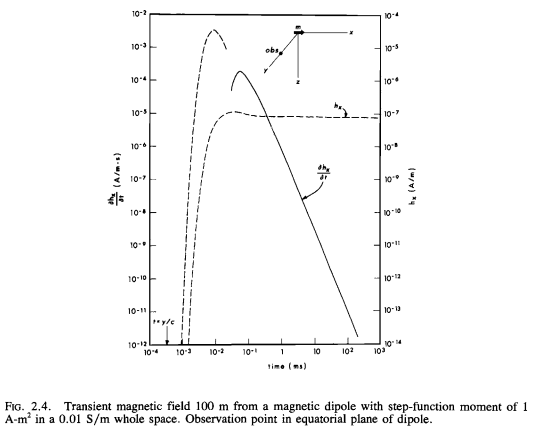
Ward and Hohmann, 1988, Fig 2.4
# Survey parameters
time = np.logspace(-7, 0, 301)
src = [0, 0, 0, 0, 0]
rec = [0, 100, 0, 0, 0]
depth = []
res = 100

# Computation
inp = {'src': src, 'rec': rec, 'depth': depth, 'res': res,
       'xdirect': True, 'freqtime': time, 'verb': 1}
fhz_num = empymod.loop(signal=1, **inp)
fdhz_num = empymod.loop(signal=0, **inp)

# Figure
plt.figure(figsize=(5, 5))

ax1 = plt.subplot(111)

plt.plot(time*1e3, fdhz_num, 'C0-', label='dHz/dt')
plt.plot(time*1e3, -fdhz_num, 'C0--')

plt.xscale('log')
plt.yscale('log')
plt.xlim([1e-4, 1e3])
plt.yticks(10**np.arange(-12., -1))
plt.ylim([1e-12, 1e-2])
plt.xlabel('time (ms)')
plt.ylabel(r'$\frac{\partial h_{\rho}}{\partial t}$ (A/m-s)')
plt.legend(loc=8)

ax2 = ax1.twinx()

plt.plot(time*1e3, fhz_num, 'C1-', label='Hz')
plt.plot(time*1e3, -fhz_num, 'C1--')

plt.xscale('log')
plt.yscale('log')
plt.xlim([1e-4, 1e3])
plt.yticks(10**np.arange(-14., -3))
plt.ylim([1e-14, 1e-4])
plt.ylabel(r'$h_{\rho}$ (A/m)')
plt.legend(loc=5)

plt.tight_layout()
plt.show()
Original Figure
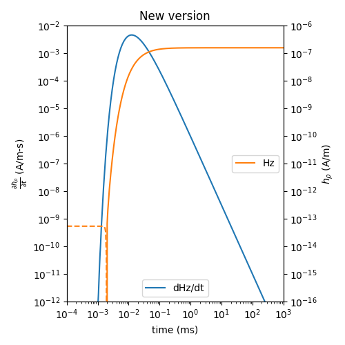
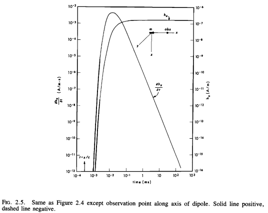
Ward and Hohmann, 1988, Fig 2.5
# Survey parameters
time = np.logspace(-7, 0, 301)
src = [0, 0, 0, 0, 0]
rec = [100, 0, 0, 0, 0]
depth = []
res = 100

# Computation
inp = {'src': src, 'rec': rec, 'depth': depth, 'res': res,
       'xdirect': True, 'freqtime': time, 'verb': 1}
fhz_num = empymod.loop(signal=1, **inp)
fdhz_num = empymod.loop(signal=0, **inp)

# Figure
plt.figure(figsize=(5, 5))

ax1 = plt.subplot(111)
plt.title('New version')

plt.plot(time*1e3, fdhz_num, 'C0-', label='dHz/dt')
plt.plot(time*1e3, -fdhz_num, 'C0--')

plt.xscale('log')
plt.yscale('log')
plt.xlim([1e-4, 1e3])
plt.yticks(10**np.arange(-12., -1))
plt.ylim([1e-12, 1e-2])
plt.xlabel('time (ms)')
plt.ylabel(r'$\frac{\partial h_{\rho}}{\partial t}$ (A/m-s)')
plt.legend(loc=8)

ax2 = ax1.twinx()

plt.plot(time*1e3, fhz_num, 'C1-', label='Hz')
plt.plot(time*1e3, -fhz_num, 'C1--')

plt.xscale('log')
plt.yscale('log')
plt.xlim([1e-4, 1e3])
plt.yticks(10**np.arange(-16., -5))
plt.ylim([1e-16, 1e-6])
plt.ylabel(r'$h_{\rho}$ (A/m)')
plt.legend(loc=5)

plt.tight_layout()
plt.show()
Original Figure
empymod.Report()
Total running time of the script: ( 0 minutes 8.819 seconds)
Estimated memory usage: 9 MB