Note
Click here to download the full example code
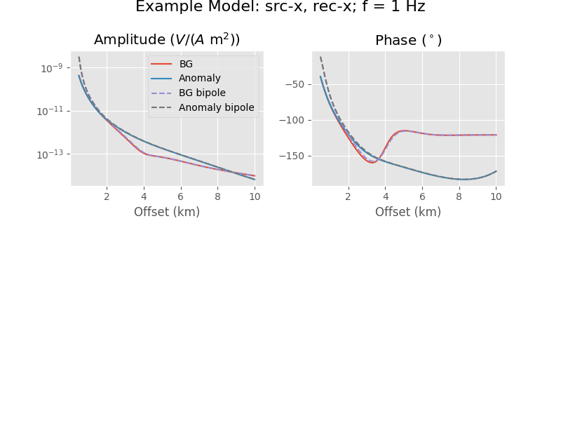
Point dipole vs finite length dipole
Comparison of a 800 m long bipole with a dipole at its centre.
import empymod
import numpy as np
import matplotlib.pyplot as plt
plt.style.use('ggplot')
Define models
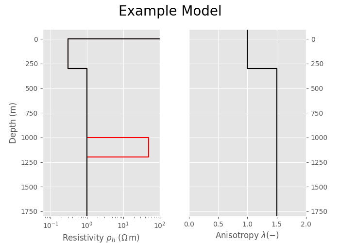
name = 'Example Model'         # Model name
depth = [0, 300, 1000, 1200]   # Layer boundaries
res = [2e14, 0.3, 1, 50, 1]    # Anomaly resistivities
resBG = [2e14, 0.3, 1, 1, 1]   # Background resistivities
aniso = [1, 1, 1.5, 1.5, 1.5]  # Layer anis. (same for anomaly and background)

# Modelling parameters
verb = 2

# Spatial parameters
zsrc = 250                   # Src-depth
zrec = 300                   # Rec-depth
fx = np.arange(5, 101)*100   # Offsets
fy = np.zeros(fx.size)       # 0s
Plot models
pdepth = np.repeat(np.r_[-100, depth], 2)
pdepth[:-1] = pdepth[1:]
pdepth[-1] = 2*depth[-1]
pres = np.repeat(res, 2)
presBG = np.repeat(resBG, 2)
pani = np.repeat(aniso, 2)

# Create figure
fig = plt.figure(figsize=(7, 5), facecolor='w')
fig.subplots_adjust(wspace=.25, hspace=.4)
plt.suptitle(name, fontsize=20)

# Plot Resistivities
ax1 = plt.subplot(1, 2, 1)
plt.plot(pres, pdepth, 'r')
plt.plot(presBG, pdepth, 'k')
plt.xscale('log')
plt.xlim([.2*np.array(res).min(), 2*np.array(res)[1:].max()])
plt.ylim([1.5*depth[-1], -100])
plt.ylabel('Depth (m)')
plt.xlabel(r'Resistivity $\rho_h\ (\Omega\,\rm{m})$')

# Plot anisotropies
ax2 = plt.subplot(1, 2, 2)
plt.plot(pani, pdepth, 'k')
plt.xlim([0, 2])
plt.ylim([1.5*depth[-1], -100])
plt.xlabel(r'Anisotropy $\lambda (-)$')
ax2.yaxis.tick_right()

plt.show()
Frequency response for f = 1 Hz
Compute
# Dipole
inpdat = {'src': [0, 0, zsrc, 0, 0], 'rec': [fx, fy, zrec, 0, 0],
          'depth': depth, 'freqtime': 1, 'aniso': aniso,
          'htarg': {'pts_per_dec': -1}, 'verb': verb}
fEM = empymod.bipole(**inpdat, res=res)
fEMBG = empymod.bipole(**inpdat, res=resBG)

# Bipole
inpdat['src'] = [-400, 400, 0, 0, zsrc, zsrc]
inpdat['srcpts'] = 10
fEMbp = empymod.bipole(**inpdat, res=res)
fEMBGbp = empymod.bipole(**inpdat, res=resBG)
Out:
:: empymod END; runtime = 0:00:16.425238 :: 1 kernel call(s)


:: empymod END; runtime = 0:00:00.003937 :: 1 kernel call(s)


:: empymod END; runtime = 0:00:00.024010 :: 10 kernel call(s)


:: empymod END; runtime = 0:00:00.023946 :: 10 kernel call(s)
Plot
fig = plt.figure(figsize=(8, 6), facecolor='w')
fig.subplots_adjust(wspace=.25, hspace=.4)
fig.suptitle(name+': src-x, rec-x; f = 1 Hz', fontsize=16, y=1)

# Plot Amplitude
ax1 = plt.subplot(2, 2, 1)
plt.semilogy(fx/1000, fEMBG.amp(), label='BG')
plt.semilogy(fx/1000, fEM.amp(), label='Anomaly')
plt.semilogy(fx/1000, fEMBGbp.amp(), '--', label='BG bipole')
plt.semilogy(fx/1000, fEMbp.amp(), '--', label='Anomaly bipole')
plt.legend(loc='best')
plt.title(r'Amplitude ($V/(A\ $m$^2$))')
plt.xlabel('Offset (km)')

# Plot Phase
ax2 = plt.subplot(2, 2, 2)
plt.title(r'Phase ($^\circ$)')
plt.plot(fx/1000, fEMBG.pha(deg=True), label='BG')
plt.plot(fx/1000, fEM.pha(deg=True), label='Anomaly')
plt.plot(fx/1000, fEMBGbp.pha(deg=True), '--', label='BG bipole')
plt.plot(fx/1000, fEMbp.pha(deg=True), '--', label='Anomaly bipole')
plt.xlabel('Offset (km)')

plt.show()
empymod.Report()
Total running time of the script: ( 0 minutes 17.855 seconds)
Estimated memory usage: 103 MB