Note
Click here to download the full example code
Ziolkowski et al., 2007
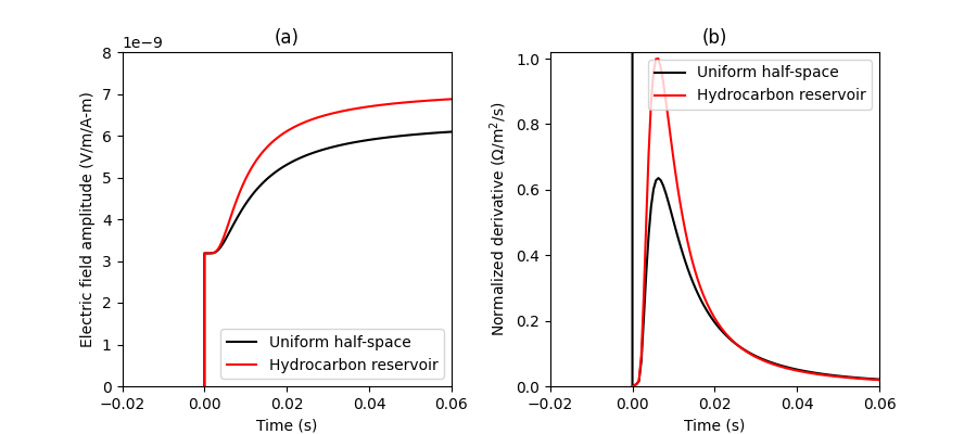
Reproducing Figure 3 of Ziolkowski et al., 2007, Geophysics. This is a land MTEM example.
Reference
Ziolkowski, A., B. Hobbs, and D. Wright, 2007, Multitransient electromagnetic demonstration survey in France: Geophysics, 72, F197-F209; DOI: 10.1190/1.2735802.
import empymod
import numpy as np
from copy import deepcopy as dc
import matplotlib.pyplot as plt
Computation
# Time
t = np.linspace(0.001, 0.06, 101)

# Target model
inp2 = {'src': [0, 0, 0.001],
        'rec': [1000, 0, 0.001],
        'depth': [0, 500, 525],
        'res': [2e14, 20, 500, 20],
        'freqtime': t,
        'verb': 1}

# HS model
inp1 = dc(inp2)
inp1['depth'] = inp2['depth'][0]
inp1['res'] = inp2['res'][:2]

# Compute responses
sths = empymod.dipole(**inp1, signal=1)  # Step, HS
sttg = empymod.dipole(**inp2, signal=1)  # " "   Target
imhs = empymod.dipole(**inp1, signal=0, ft='fftlog')  # Impulse, HS
imtg = empymod.dipole(**inp2, signal=0, ft='fftlog')  # " "      Target
Plot
plt.figure(figsize=(9, 4))
plt.subplots_adjust(wspace=.3)

# Step response
plt.subplot(121)
plt.title('(a)')
plt.plot(np.r_[0, 0, t], np.r_[0, sths[0], sths], 'k',
         label='Uniform half-space')
plt.plot(np.r_[0, 0, t], np.r_[0, sttg[0], sttg], 'r',
         label='Hydrocarbon reservoir')
plt.axis([-.02, 0.06, 0, 8e-9])
plt.xlabel('Time (s)')
plt.ylabel('Electric field amplitude (V/m/A-m)')
plt.legend()

# Impulse response
plt.subplot(122)
plt.title('(b)')

# Normalize by max-response
ntg = np.max(np.r_[imtg, imhs])

plt.plot(np.r_[0, 0, t], np.r_[2, 0, imhs/ntg], 'k',
         label='Uniform half-space')
plt.plot(np.r_[0, t], np.r_[0, imtg/ntg], 'r', label='Hydrocarbon reservoir')
plt.axis([-.02, 0.06, 0, 1.02])
plt.xlabel('Time (s)')
plt.ylabel(r'Normalized derivative ($\Omega$/m$^2$/s)')
plt.legend()
plt.show()
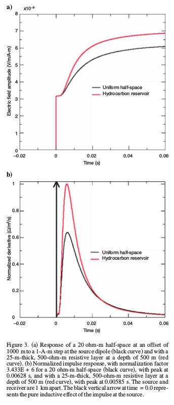
Original Figure
Figure 3 of Ziolkowski et al., 2007, Geophysics:
empymod.Report()
Total running time of the script: ( 0 minutes 1.341 seconds)
Estimated memory usage: 9 MB