Note
Click here to download the full example code
Constable and Weiss, 2006
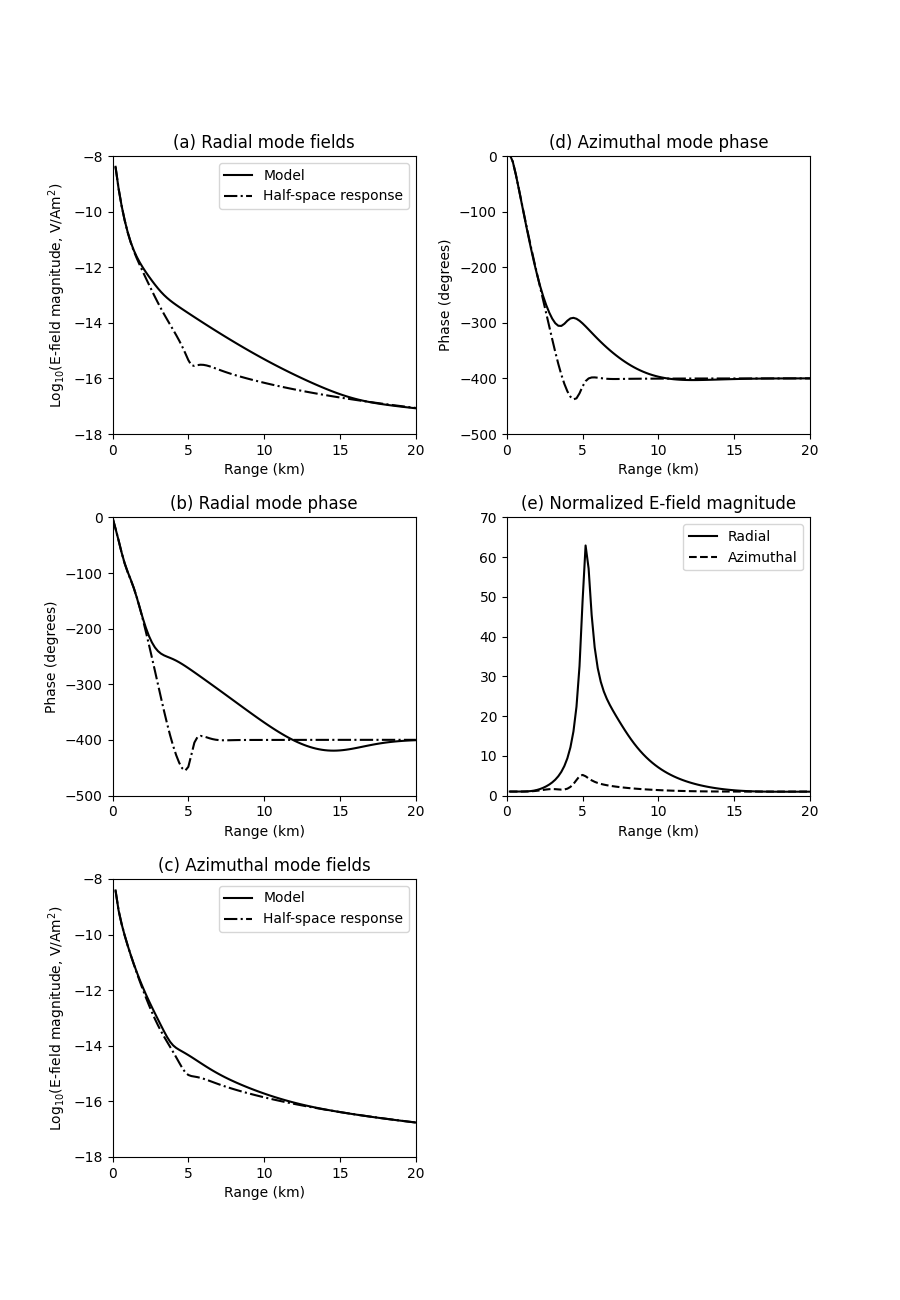
Reproducing Figure 3 of Constable and Weiss, 2006, Geophysics. This is a marine CSEM example.
Reference
Constable, S., and C. J. Weiss, 2006, Mapping thin resistors and hydrocarbons with marine EM methods: Insights from 1D modeling: Geophysics, 71, G43-G51; DOI: 10.1190/1.2187748.
import empymod
import numpy as np
from copy import deepcopy as dc
import matplotlib.pyplot as plt
Computation
Note: Exact reproduction is not possible, as source and receiver depths are not explicitly specified in the publication. I made a few checks, and it looks like a source-depth of 900 meter gives good accordance. Receivers are on the sea-floor.
# Offsets
x = np.linspace(0, 20000, 101)

# TG model
inp3 = {'src': [0, 0, 900],
        'rec': [x, np.zeros(x.shape), 1000],
        'depth': [0, 1000, 2000, 2100],
        'res': [2e14, 0.3, 1, 100, 1],
        'freqtime': 1,
        'verb': 1}

# HS model
inp4 = dc(inp3)
inp4['depth'] = inp3['depth'][:2]
inp4['res'] = inp3['res'][:3]

# Compute radial responses
rhs = empymod.dipole(**inp4)  # Step, HS
rhs = empymod.utils.EMArray(np.nan_to_num(rhs))
rtg = empymod.dipole(**inp3)  # " "   Target
rtg = empymod.utils.EMArray(np.nan_to_num(rtg))

# Compute azimuthal response
ahs = empymod.dipole(**inp4, ab=22)  # Step, HS
ahs = empymod.utils.EMArray(np.nan_to_num(ahs))
atg = empymod.dipole(**inp3, ab=22)  # " "   Target
atg = empymod.utils.EMArray(np.nan_to_num(atg))
Out:
* WARNING :: Offsets < 0.001 m are set to 0.001 m!
* WARNING :: Offsets < 0.001 m are set to 0.001 m!
* WARNING :: Offsets < 0.001 m are set to 0.001 m!
* WARNING :: Offsets < 0.001 m are set to 0.001 m!
Plot
plt.figure(figsize=(9, 13))
plt.subplots_adjust(wspace=.3, hspace=.3)

# Radial amplitude
plt.subplot(321)
plt.title('(a) Radial mode fields')
plt.plot(x/1000, np.log10(rtg.amp()), 'k', label='Model')
plt.plot(x/1000, np.log10(rhs.amp()), 'k-.', label='Half-space response')
plt.axis([0, 20, -18, -8])
plt.xlabel('Range (km)')
plt.ylabel(r'Log$_{10}$(E-field magnitude, V/Am$^2$)')
plt.legend()

# Radial phase
plt.subplot(323)
plt.title('(b) Radial mode phase')
plt.plot(x/1000, rtg.pha(deg=True), 'k')
plt.plot(x/1000, rhs.pha(deg=True), 'k-.')
plt.axis([0, 20, -500, 0])
plt.xlabel('Range (km)')
plt.ylabel('Phase (degrees)')

# Azimuthal amplitude
plt.subplot(325)
plt.title('(c) Azimuthal mode fields')
plt.plot(x/1000, np.log10(atg.amp()), 'k', label='Model')
plt.plot(x/1000, np.log10(ahs.amp()), 'k-.', label='Half-space response')
plt.axis([0, 20, -18, -8])
plt.xlabel('Range (km)')
plt.ylabel(r'Log$_{10}$(E-field magnitude, V/Am$^2$)')
plt.legend()

# Azimuthal phase
plt.subplot(322)
plt.title('(d) Azimuthal mode phase')
plt.plot(x/1000, atg.pha(deg=True)+180, 'k')
plt.plot(x/1000, ahs.pha(deg=True)+180, 'k-.')
plt.axis([0, 20, -500, 0])
plt.xlabel('Range (km)')
plt.ylabel('Phase (degrees)')

# Normalized
plt.subplot(324)
plt.title('(e) Normalized E-field magnitude')
plt.plot(x/1000, np.abs(rtg/rhs), 'k', label='Radial')
plt.plot(x/1000, np.abs(atg/ahs), 'k--', label='Azimuthal')
plt.axis([0, 20, 0, 70])
plt.xlabel('Range (km)')
plt.legend()

plt.show()
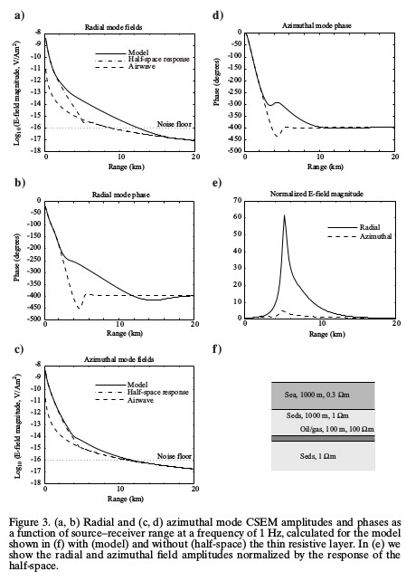
Original Figure
Figure 3 of Constable and Weiss, 2006, Geophysics:
empymod.Report()
Total running time of the script: ( 0 minutes 1.364 seconds)
Estimated memory usage: 17 MB