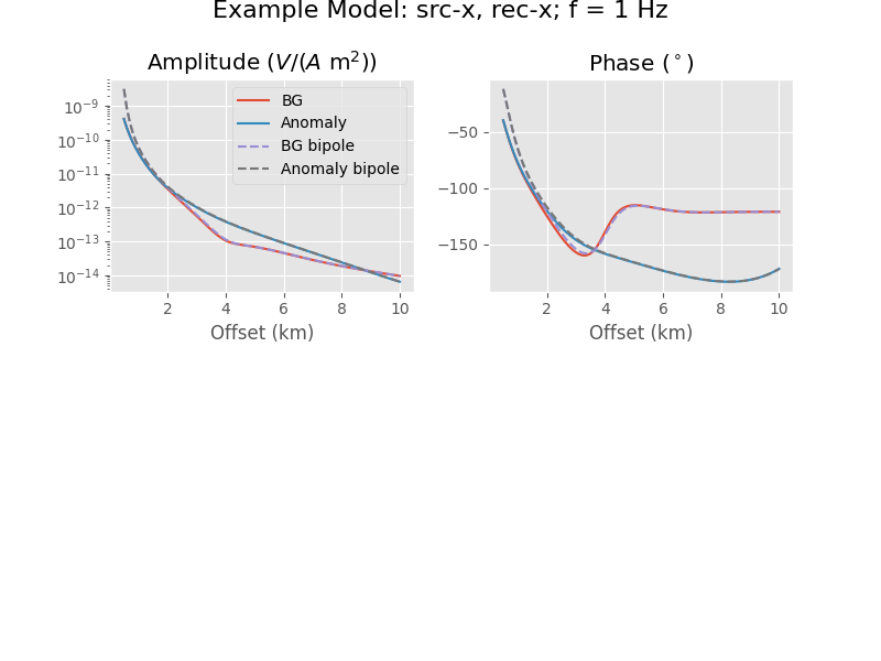
Point dipole vs finite length dipole#

Comparison of the Eₓₓ-fields (in-line electric x-directed field generated by an electric x-directed source) between a

800 m long bipole source, and a
infinitesimal small (point) dipole source,

where the latter is located at the center of the former.

A common rule of thumb ¹ is that a finite length bipole can be approximated by an infinitesimal small dipole, if the receivers are further away than five times the bipole length. In this case, this would be from 4 km onwards (five times 800 m).

¹ See, e.g., page 288 of Spies, B. R., and F. C. Frischknecht, 1991, Electromagnetic sounding: SEG, Investigations in Geophysics, No. 3, 5, 285-425; DOI 10.1190/1.9781560802686. There it was used to approximate a loop as a magnetic point dipole, but similar approximations are used for finite vs point electric dipoles.

import empymod
import numpy as np
import matplotlib.pyplot as plt
plt.style.use('ggplot')

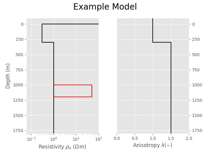
Define models#

depth = [0, -300, -1000, -1200]  # Layer boundaries
res_tg = [2e14, 0.3, 1, 50, 1]   # Anomaly resistivities
res_bg = [2e14, 0.3, 1, 1, 1]    # Background resistivities
aniso = [1, 1, 1.5, 1.5, 1.5]    # Layer anisotropies (same for entire model)

Plot models#

p_depth = np.repeat(np.r_[100, depth, 2*depth[-1]], 2)[1:-1]

# Create figure
fig, (ax1, ax2) = plt.subplots(1, 2, constrained_layout=True, sharey=True)
fig.suptitle("Model", fontsize=16)

# Plot Resistivities
ax1.semilogx(np.repeat(res_tg, 2), p_depth, 'C0')
ax1.semilogx(np.repeat(res_bg, 2), p_depth, 'k')
ax1.set_xlim([0.08, 500])
ax1.set_ylim([-1800, 100])
ax1.set_ylabel('Depth (m)')
ax1.set_xlabel('Resistivity ρₕ (Ωm)')

# Plot anisotropies
ax2.plot(np.repeat(aniso, 2), p_depth, 'k')
ax2.set_xlim([0, 2])
ax2.set_xlabel('Anisotropy λ (-)')
ax2.yaxis.tick_right()

Frequency response for f = 1 Hz#

Compute#

# Spatial parameters
srcz = -250                   # Source depth
recz = -300                   # Receiver depth
recx = np.arange(5, 101)*100  # Receiver offsets in x-direction
recy = np.zeros(96)           # Receiver offsets in y-direction

# General input
inpdat = {
    'rec': [recx, recy, recz, 0, 0],
    'depth': depth,
    'freqtime': 1,                 # 1 Hz
    'aniso': aniso,
    'htarg': {'pts_per_dec': -1},  # Faster computation
    'verb': 2,                     # Verbosity
}

# Dipole Source [x, y, z, azm, dip]
inpdat['src'] = [0, 0, srcz, 0, 0]
dip_tg = empymod.bipole(res=res_tg, **inpdat)
dip_bg = empymod.bipole(res=res_bg, **inpdat)

# Bipole Source [ x0,  x1, y0, y1,  z0,   z1]
inpdat['src'] = [-400, 400, 0, 0, srcz, srcz]
inpdat['srcpts'] = 10  # Bipole computed with 10 dipoles
bip_tg = empymod.bipole(res=res_tg, **inpdat)
bip_bg = empymod.bipole(res=res_bg, **inpdat)

:: empymod END; runtime = 0:00:12.686168 :: 1 kernel call(s)

:: empymod END; runtime = 0:00:00.001462 :: 1 kernel call(s)

:: empymod END; runtime = 0:00:00.010147 :: 10 kernel call(s)

:: empymod END; runtime = 0:00:00.009372 :: 10 kernel call(s)

Plot#

fig, (ax1, ax2) = plt.subplots(2, 1, sharex=True, constrained_layout=True)

ax1.set_title("Eₓₓ; f = 1 Hz")

# Plot Amplitude
ax1.semilogy(recx/1000, dip_bg.amp())
ax1.semilogy(recx/1000, dip_tg.amp())
ax1.semilogy(recx/1000, bip_bg.amp(), '--')
ax1.semilogy(recx/1000, bip_tg.amp(), '--')
ax1.set_ylabel('Amplitude (V/(Am²))')

# Plot Phase
ax2.plot(recx/1000, dip_bg.pha(deg=True), label='Dipole: background')
ax2.plot(recx/1000, dip_tg.pha(deg=True), label='Dipole: anomaly')
ax2.plot(recx/1000, bip_bg.pha(deg=True), '--', label='Bipole: background')
ax2.plot(recx/1000, bip_tg.pha(deg=True), '--', label='Bipole: target')
ax2.set_xlabel('Offset (km)')
ax2.set_ylabel('Phase (°)')
ax2.legend(ncols=2, loc='upper center')

empymod.Report()

Wed Mar 12 21:10:23 2025 UTC
OS	Linux (Ubuntu 22.04)	CPU(s)	2	Machine	x86_64
Architecture	64bit	RAM	7.6 GiB	Environment	Python
File system	ext4
Python 3.11.10 (main, Nov 5 2024, 16:13:19) [GCC 11.4.0]
numpy	2.1.3	scipy	1.15.2	numba	0.61.0
empymod	2.5.1	libdlf	0.3.0	IPython	9.0.2
matplotlib	3.10.1