Note
Go to the end to download the full example code.
Difference between magnetic dipole and loop sources#
In this example we look at the differences between an electric loop loop, which results in a magnetic source, and a magnetic dipole source.
The derivation of the electromagnetic field in Hunziker et al. (2015) is for electric and magnetic point-dipole sources and receivers. The magnetic field due to a magnetic source (\(mm\)) is obtain from the electric field due to an electric source (\(ee\)) using the duality principle, given in their Equation (11),
Without going into the details of the different parameters, we can focus on the difference between the \(mm\) and \(ee\) fields for a homogeneous, isotropic fullspace by simplifying this further to
Here, \(\sigma\) is conductivity (S/m), \(\omega=2\pi f\) is angular frequency (Hz), and \(\mu\) is the magnetic permeability (H/m). So from Equation (2) we see that the \(mm\) field differs from the \(ee\) field by a factor \(\sigma/(\mathrm{i}\omega\mu)\).
A magnetic dipole source has a moment of \(I^mds\); however, a magnetic dipole source is basically never used in geophysics. Instead a loop of an electric wire is used, which generates a magnetic field. The moment generated by this loop is given by \(I^m = \mathrm{i}\omega\mu N A I^e\), where \(A\) is the area of the loop (m:math:^2), and \(N\) the number of turns of the loop. So the difference between a unit magnetic dipole and a unit loop (\(A=1, N=1\)) is the factor \(\mathrm{i}\omega\mu\), hence Equation (2) becomes
This notebook shows this relation in the frequency domain, as well as for impulse, step-on, and step-off responses in the time domain.
We can actually model an electric loop instead of adjusting the magnetic dipole solution to correspond to a loop source. This is shown in the second part of the notebook.
References
Hunziker, J., J. Thorbecke, and E. Slob, 2015, The electromagnetic response in a layered vertical transverse isotropic medium: A new look at an old problem: Geophysics, 80(1), F1–F18; DOI: 10.1190/geo2013-0411.1.
import empymod
import numpy as np
import matplotlib.pyplot as plt
plt.style.use('ggplot')
1. Using the magnetic dipole solution#
Survey parameters#
Homogenous fullspace of \(\sigma\) = 0.01 S/m.
Source at the origin, x-directed.
Inline receiver with offset of 100 m, x-directed.
freq = np.logspace(-1, 5, 301)  # Frequencies (Hz)
time = np.logspace(-6, 0, 301)  # Times (s)
src = [0, 0, 0, 0, 0]    # x-dir. source at the origin [x, y, z, azimuth, dip]
rec = [100, 0, 0, 0, 0]  # x-dir. receiver 100m away from source, inline
cond = 0.01              # Conductivity (S/m)
Computation using empymod#
# Collect common parameters
inp = {'src': src, 'rec': rec, 'depth': [], 'res': 1/cond, 'verb': 1}

# Frequency domain
inp['freqtime'] = freq
fee_dip_dip = empymod.bipole(**inp)
fmm_dip_dip = empymod.bipole(msrc=True, mrec=True, **inp)
f_loo_dip = empymod.bipole(msrc='b', mrec=True, **inp)

# Time domain
inp['freqtime'] = time

# ee
ee_dip_dip_of = empymod.bipole(signal=-1, **inp)
ee_dip_dip_im = empymod.bipole(signal=0, **inp)
ee_dip_dip_on = empymod.bipole(signal=1, **inp)

# mm dip-dip
dip_dip_of = empymod.bipole(signal=-1, msrc=True, mrec=True, **inp)
dip_dip_im = empymod.bipole(signal=0, msrc=True, mrec=True, **inp)
dip_dip_on = empymod.bipole(signal=1, msrc=True, mrec=True, **inp)

# mm loop-dip
loo_dip_of = empymod.bipole(msrc='b', mrec=True, signal=-1, **inp)
loo_dip_im = empymod.bipole(msrc='b', mrec=True, signal=0, **inp)
loo_dip_on = empymod.bipole(msrc='b', mrec=True, signal=1, **inp)
Plot the result#
fs = 16  # Fontsize

# Figure
fig = plt.figure(figsize=(12, 8), constrained_layout=True)

# Frequency Domain
plt.subplot(231)
plt.title(r'$G^{ee}_{\rm{dip-dip}}$', fontsize=fs)
plt.plot(freq, fee_dip_dip.real, 'C0-', label='Real')
plt.plot(freq, -fee_dip_dip.real, 'C0--')
plt.plot(freq, fee_dip_dip.imag, 'C1-', label='Imag')
plt.plot(freq, -fee_dip_dip.imag, 'C1--')
plt.xscale('log')
plt.yscale('log')
plt.ylim([5e-8, 2e-5])

ax1 = plt.subplot(232)
plt.title(r'$G^{mm}_{\rm{dip-dip}}$', fontsize=fs)
plt.plot(freq, fmm_dip_dip.real, 'C0-', label='Real')
plt.plot(freq, -fmm_dip_dip.real, 'C0--')
plt.plot(freq, fmm_dip_dip.imag, 'C1-', label='Imag')
plt.plot(freq, -fmm_dip_dip.imag, 'C1--')
plt.xscale('log')
plt.yscale('log')
plt.xlabel('Frequency (Hz)', fontsize=fs-2)
plt.legend()

plt.subplot(233)
plt.title(r'$G^{mm}_{\rm{loop-dip}}$', fontsize=fs)
plt.plot(freq, f_loo_dip.real, 'C0-', label='Real')
plt.plot(freq, -f_loo_dip.real, 'C0--')
plt.plot(freq, f_loo_dip.imag, 'C1-', label='Imag')
plt.plot(freq, -f_loo_dip.imag, 'C1--')
plt.xscale('log')
plt.yscale('log')
plt.ylim([5e-10, 2e-7])

plt.text(1.05, 0.5, "Frequency Domain", {'fontsize': fs},
         horizontalalignment='left', verticalalignment='center',
         rotation=-90, clip_on=False, transform=plt.gca().transAxes)

# Time Domain
plt.subplot(234)
plt.plot(time, ee_dip_dip_of, 'C0-', label='Step-Off')
plt.plot(time, -ee_dip_dip_of, 'C0--')
plt.plot(time, ee_dip_dip_im, 'C1-', label='Impulse')
plt.plot(time, -ee_dip_dip_im, 'C1--')
plt.plot(time, ee_dip_dip_on, 'C2-', label='Step-On')
plt.plot(time, -ee_dip_dip_on, 'C2--')
plt.xscale('log')
plt.yscale('log')

plt.subplot(235)
plt.plot(time, dip_dip_of, 'C0-', label='Step-Off')
plt.plot(time, -dip_dip_of, 'C0--')
plt.plot(time, dip_dip_im, 'C1-', label='Impulse')
plt.plot(time, -dip_dip_im, 'C1--')
plt.plot(time, dip_dip_on, 'C2-', label='Step-On')
plt.plot(time, -dip_dip_on, 'C2--')
plt.xscale('log')
plt.yscale('log')
plt.xlabel('Time (s)', fontsize=fs-2)
plt.legend()

plt.subplot(236)
plt.plot(time, loo_dip_of, 'C0-', label='Step-Off')
plt.plot(time, -loo_dip_of, 'C0--')
plt.plot(time, loo_dip_im, 'C1-', label='Impulse')
plt.plot(time, -loo_dip_im, 'C1--')
plt.plot(time, loo_dip_on, 'C2-', label='Step-On')
plt.plot(time, -loo_dip_on, 'C2--')
plt.xscale('log')
plt.yscale('log')

plt.text(1.05, 0.5, "Time Domain", {'fontsize': fs},
         horizontalalignment='left', verticalalignment='center',
         rotation=-90, clip_on=False, transform=plt.gca().transAxes)

fig.text(-0.01, 0.5, 'Amplitude; e-rec (V/m); m-rec (A/m)',
         va='center', rotation='vertical', fontsize=fs, color='.4')
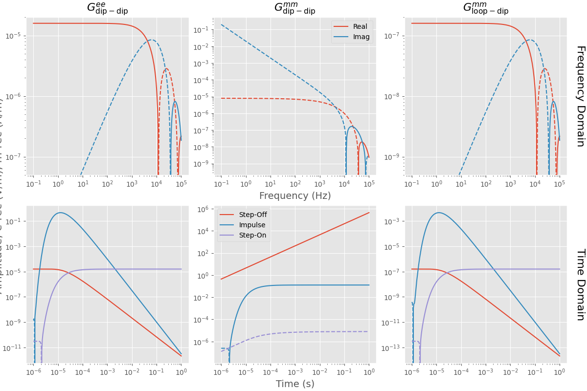
The figure shows the main points of Equations (2) and (3):
The magnetic dipole-dipole response differs by a factor \(\sigma/(\mathrm{i}\omega\mu)\) from the electric dipole-dipole response. That means for the time-domain that the magnetic response looks more like the time derivative of the electric response (e.g., the magnetic impulse responses resembles the electric step-on response).
The magnetic loop-dipole response differs only by \(\sigma\) from the electric dipole-dipole response, hence a factor of 0.01.
The units of the response only depend on the receiver, what the receiver actually measures. So if we change the source from a dipole to a loop it does not change the units of the received responses.
2. Using an electric loop#
We can use empymod to model arbitrary shaped sources by simply adding
point dipole sources together. This is what empymod does internally to
model a finite length dipole (empymod.bipole), where it uses a Gaussian
quadrature with a few points.
Here, we are going to compare the result from loop, as presented above,
with two different simulations of an electric loop source, assuming a square
loop which sides are 1 m long, so the area correspond to one square meter.
Plotting routines#
def plot_result(data1, data2, x, title, vmin=-15., vmax=-7., rx=0):
    """Plot result."""
    fig = plt.figure(figsize=(18, 10))

    def setplot(name):
        """Plot settings"""
        plt.title(name)
        plt.xlim(rx.min(), rx.max())
        plt.ylim(rx.min(), rx.max())
        plt.axis("equal")

    # Plot Re(data)
    ax1 = plt.subplot(231)
    setplot(r"(a) |Re(magn.dip*iwu)|")
    cf0 = plt.pcolormesh(rx, rx, np.log10(np.abs(data1.real)), linewidth=0,
                         rasterized=True, cmap="viridis", vmin=vmin, vmax=vmax,
                         shading='nearest')

    ax2 = plt.subplot(232)
    setplot(r"(b) |Re(el. square)|")
    plt.pcolormesh(rx, rx, np.log10(np.abs(data2.real)), linewidth=0,
                   rasterized=True, cmap="viridis", vmin=vmin, vmax=vmax,
                   shading='nearest')

    ax3 = plt.subplot(233)
    setplot(r"(c) Error real part")
    error_r = np.abs((data1.real-data2.real)/data1.real)*100
    cf2 = plt.pcolormesh(rx, rx, np.log10(error_r), vmin=-2, vmax=2,
                         linewidth=0, rasterized=True,
                         cmap=plt.get_cmap("RdBu_r", 8),
                         shading='nearest')

    # Plot Im(data)
    ax4 = plt.subplot(234)
    setplot(r"(d) |Im(magn.dip*iwu)|")
    plt.pcolormesh(rx, rx, np.log10(np.abs(data1.imag)), linewidth=0,
                   rasterized=True, cmap="viridis", vmin=vmin, vmax=vmax,
                   shading='nearest')

    ax5 = plt.subplot(235)
    setplot(r"(e) |Im(el. square)|")
    plt.pcolormesh(rx, rx, np.log10(np.abs(data2.imag)), linewidth=0,
                   rasterized=True, cmap="viridis", vmin=vmin, vmax=vmax,
                   shading='nearest')

    ax6 = plt.subplot(236)
    setplot(r"(f) Error imag part")
    error_i = np.abs((data1.imag-data2.imag)/data1.imag)*100
    plt.pcolormesh(rx, rx, np.log10(error_i), vmin=-2, vmax=2,
                   linewidth=0, rasterized=True,
                   cmap=plt.get_cmap("RdBu_r", 8),
                   shading='nearest')

    # Colorbars
    fig.colorbar(cf0, ax=[ax1, ax2, ax3], label=r"$\log_{10}$ Amplitude (A/m)")
    cbar = fig.colorbar(cf2, ax=[ax4, ax5, ax6], label=r"Relative Error")
    cbar.set_ticks([-2, -1, 0, 1, 2])
    cbar.ax.set_yticklabels([r"$0.01\,\%$", r"$0.1\,\%$", r"$1\,\%$",
                             r"$10\,\%$", r"$100\,\%$"])

    # Axis label
    fig.text(0.4, 0.05, "Inline Offset (m)", fontsize=14)
    fig.text(0.08, 0.5, 'Crossline Offset (m)', rotation=90, fontsize=14)

    # Title
    fig.suptitle(title, y=.95, fontsize=20)
Model parameters#
Resistivity: \(1 \Omega\) m fullspace
Survey#
Source at [0, 0, 0]
Receivers at [x, y, 10]
frequencies: 100 Hz.
Offsets: -250 m - 250 m
Compute empymod.loop result#
2.1 Point dipoles at (x, y) using empymod.dipole#
(0.5, 0), ab=42
(0, 0.5), ab=41
(-0.5, 0), ab=-42
(0, -0.5), ab=-41
rec_dip = [rxx, ryy, 10]
square_pts = +empymod.dipole(src=[+0.5, +0.0, 0], rec=rec_dip, ab=42,
**model).reshape(np.shape(rx))
square_pts -= empymod.dipole(src=[+0.0, +0.5, 0], rec=rec_dip, ab=41,
**model).reshape(np.shape(rx))
square_pts -= empymod.dipole(src=[-0.5, +0.0, 0], rec=rec_dip, ab=42,
**model).reshape(np.shape(rx))
square_pts += empymod.dipole(src=[+0.0, -0.5, 0], rec=rec_dip, ab=41,
**model).reshape(np.shape(rx))
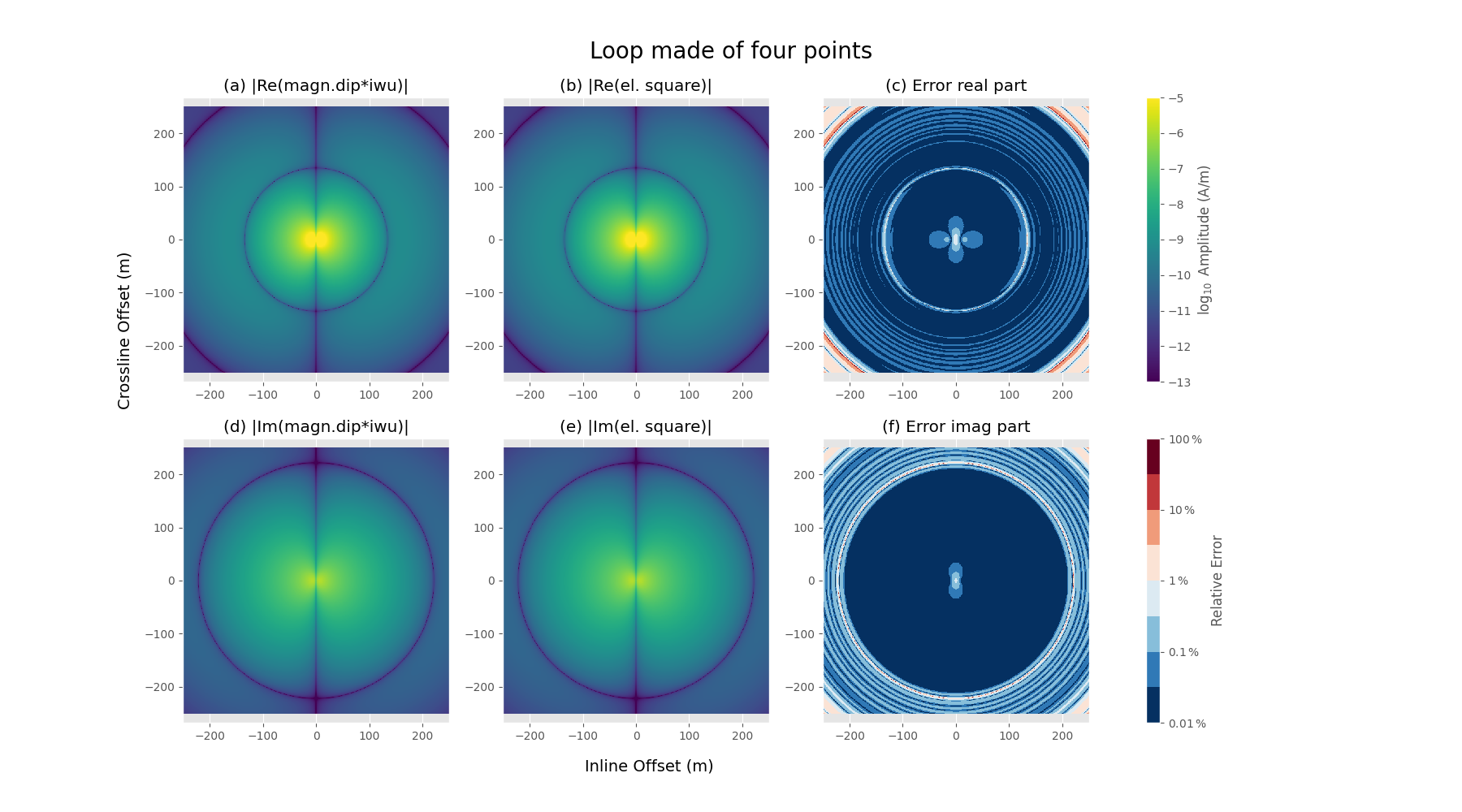
plot_result(epm_loop, square_pts, x, 'Loop made of four points',
vmin=-13, vmax=-5, rx=x)
2.2 Finite length dipoles using empymod.bipole#
Each simulated with a 5pt Gaussian quadrature. The dipoles are:
(-0.5, -0.5) to (+0.5, -0.5)
(+0.5, -0.5) to (+0.5, +0.5)
(+0.5, +0.5) to (-0.5, +0.5)
(-0.5, +0.5) to (-0.5, -0.5)
inp_dip = {
    'rec': [rxx, ryy, 10, 0, 0],
    'mrec': True,
    'srcpts': 5  # Gaussian quadr. with 5 pts to simulate a finite length dip.
}

square_dip = +empymod.bipole(src=[+0.5, +0.5, -0.5, +0.5, 0, 0],
                             **inp_dip, **model)
square_dip += empymod.bipole(src=[+0.5, -0.5, +0.5, +0.5, 0, 0],
                             **inp_dip, **model)
square_dip += empymod.bipole(src=[-0.5, -0.5, +0.5, -0.5, 0, 0],
                             **inp_dip, **model)
square_dip += empymod.bipole(src=[-0.5, +0.5, -0.5, -0.5, 0, 0],
                             **inp_dip, **model)
square_dip = square_dip.reshape(np.shape(rx))

plot_result(epm_loop, square_dip, x, 'Loop made of four dipoles',
            vmin=-13, vmax=-5, rx=x)
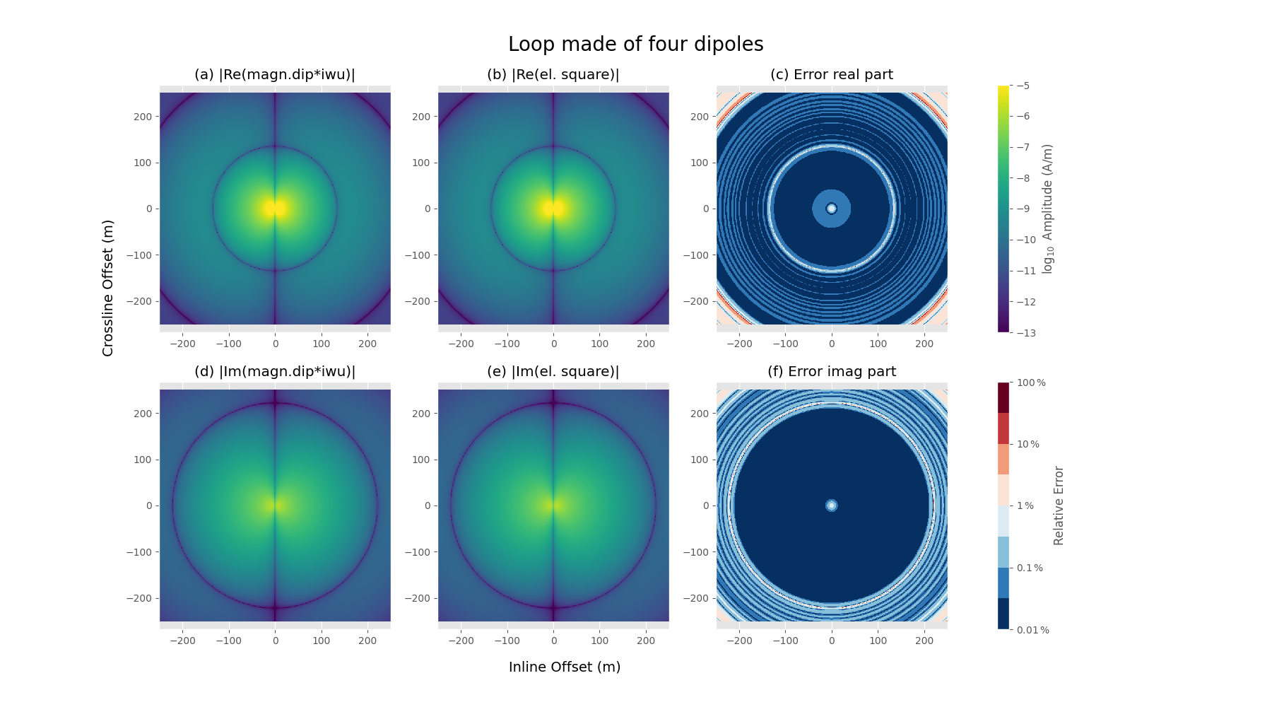
Close to the source the results between
a magnetic dipole,
an electric loop conisting of four point sources, and
an electric loop consisting of four finite length dipoles,
differ, as expected. However, for the vast majority they are identical. Skin depth for our example with \(\rho=1\Omega\) m and \(f=100\) Hz is roughly 50 m, so the results are basically identical for 4-5 skin depths, after which the signal is very low.
empymod.Report()
Total running time of the script: (0 minutes 5.574 seconds)
Estimated memory usage: 387 MB