Note
Go to the end to download the full example code.
Magnetotelluric data#
The magnetotelluric (MT) method is a passive method using as a source variations in Earth’s magnetic field, which create telluric currents in the Earth. The variation of Earth’s magnetic field has many origins, e.g., lightning or the interaction between the Earth’s magnetic field and solar wind.
Ubiquitous in MT is the plane-wave approximation, hence, that the source signal is a plane wave hitting the Earth’s surface. Having a 1D source (vertical plane wave) for a layered, 1D model reduces the computation of the impedances and from there to the apparent resistivity and apparent phase to a simple recursion algorithm. As such it does not make sense to use a full EM wavefield algorithm with three-dimensional sources such as empymod to compute MT responses. However, it is still interesting to see if we can compute MT impedances with a three-dimensional point source.
As background theory we reproduce here Equations (11) to (17) from Pedersen and Hermance (1986), with surrounding text. For a more in-depth read we refer to Chave and Jones (2012).
If we define the impedance as
[…] we can develop a recursive relationship for the impedance at the top of the j-th layer looking down
where
and the impedance at the surface of the deepest layer (\(j=N\)) is given by
The surface impedance, \(Z_j\), is found by applying Equation (2) recursively from the top of the bottom half-space, \(j = N\), and propagating upwards. From the surface impedance, \(Z_1\), we can then calculate the apparent resistivity, \(\rho_a\), and phase, \(\theta_a\), as
This calculation is repeated for a range of periods and is used to model the magnetotelluric response of the layered structure.
Note that in this example we assume that positive z points upwards.
Reference:
Chave, A., and Jones, A. (Eds.), 2012. The Magnetotelluric Method: Theory and Practice. Cambridge: Cambridge University Press; DOI: 10.1017/CBO9781139020138.
Pedersen, J., and Hermance, J.F., 1986. Least squares inversion of one-dimensional magnetotelluric data: An assessment of procedures employed by Brown University. Surveys in Geophysics 8, 187–231 (1986); DOI: 10.1007/BF01902413.
This example was strongly motivated by Andrew Pethicks blog post tutorial-1d-mt-forward.
import empymod
import numpy as np
import matplotlib.pyplot as plt
from scipy.constants import mu_0
plt.style.use('ggplot')
Define model parameter and frequencies#
resistivities = np.array([2e14, 300, 2500, 0.8, 3000, 2500])
depths = np.array([0, -200, -600, -640, -1140])
frequencies = np.logspace(-4, 5, 101)
omega = 2 * np.pi * frequencies
1D-MT recursion following Pedersen & Hermance#
Using the variable names as in the paper.
# Initiate recursive formula with impedance of the deepest layer.
Z_j = np.sqrt(1j * omega * mu_0 * resistivities[-1])

# Move up the stack of layers till the top (without air).
for j in range(depths.size-1, 0, -1):

    # Thickness
    t_j = depths[j-1] - depths[j]

    # Intrinsic impedance
    z_oj = np.sqrt(1j * omega * mu_0 * resistivities[j])

    # Reflection coefficient
    R_j = (z_oj - Z_j) / (z_oj + Z_j)

    # Exponential factor
    gamma_j = np.sqrt(1j * omega * mu_0 / resistivities[j])
    exp_j = np.exp(-2 * gamma_j * t_j)

    # Impedance at this layer
    Z_j = z_oj * (1 - R_j * exp_j) / (1 + R_j * exp_j)

# Step 3. Compute apparent resistivity last impedance
apres_mt1d = abs(Z_j)**2/(omega * mu_0)
phase_mt1d = np.arctan2(Z_j.imag, Z_j.real)
1D MT using empymod#
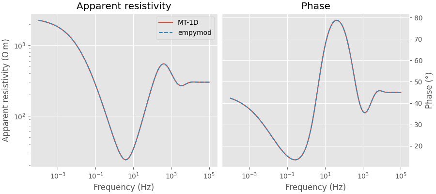
The above derivation and code assume plane waves. We can “simulate” plane waves by putting the source _very_ far away. In this example, we set it one million km away in all directions. As the impedance is the ratio of the Ex and Hy fields the source type (electric or magnetic) and the source orientation do not matter; hence, it can be an arbitrarily rotated electric or magnetic source, the apparent resistivity and apparent phase will always be the same.
dist = 1_000_000_000  # 1 million kilometer (!)
inp = {
    'src': (dist, dist, dist),
    'rec': (0, 0, -0.1),
    'res': resistivities,
    'depth': depths,
    'freqtime': frequencies,
    'verb': 1,
}

# Get Ex, Hy.
ex = empymod.dipole(ab=11, **inp)
hy = -empymod.dipole(ab=51, **inp)

# Impedance.
Z = ex/hy

# Apparent resistivity and apparent phase.
apres_empy = abs(Z)**2 / (omega * mu_0)
phase_empy = np.arctan2(Z.imag, Z.real)
Plot results#
fig, (ax1, ax2) = plt.subplots(1, 2, figsize=(9, 4), constrained_layout=True)

ax1.set_title('Apparent resistivity')
ax1.loglog(frequencies, apres_mt1d, label='MT-1D')
ax1.loglog(frequencies, apres_empy, '--', label='empymod')
ax1.set_xlabel('Frequency (Hz)')
ax1.set_ylabel('Apparent resistivity (Ω m)')
ax1.legend()

ax2.set_title('Phase')
ax2.semilogx(frequencies, phase_mt1d*180/np.pi)
ax2.semilogx(frequencies, phase_empy*180/np.pi, '--')
ax2.yaxis.tick_right()
ax2.set_xlabel('Frequency (Hz)')
ax2.set_ylabel('Phase (°)')
ax2.yaxis.set_label_position("right")
empymod.Report()
Total running time of the script: (0 minutes 0.961 seconds)
Estimated memory usage: 194 MB