A simple frequency-domain example

A simple frequency-domain empymod example for a

• single frequency, and a

• crossplot of a range of frequencies versus a range of offsets.

import empymod
import numpy as np
import matplotlib.pyplot as plt
plt.style.use('ggplot')

Define models

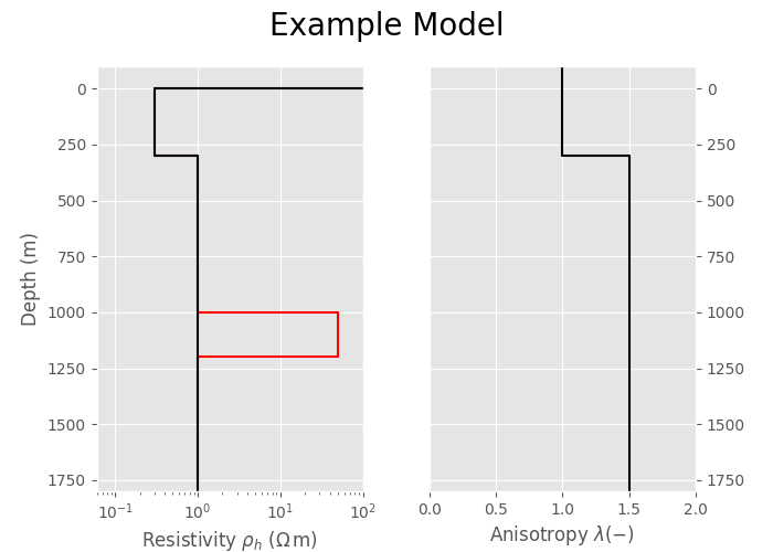
depth = [0, -300, -1000, -1200]   # Layer boundaries
res_tg = [2e14, 0.3, 1, 50, 1]    # Anomaly resistivities
res_bg = [2e14, 0.3, 1, 1, 1]     # Background resistivities
aniso = [1, 1, 1.5, 1.5, 1.5]     # Layer anis. (same for anomaly & backg.)

# Modelling parameters
verb = 0
ab = 11   # source and receiver x-directed

# Spatial parameters
zsrc = -250                     # Source depth
zrec = -300                     # Receiver depth
recx = np.arange(20, 101)*100   # Receiver offsets

Plot models

p_depth = np.repeat(np.r_[100, depth, 2*depth[-1]], 2)[1:-1]

# Create figure
fig, (ax1, ax2) = plt.subplots(1, 2, constrained_layout=True, sharey=True)
fig.suptitle("Model", fontsize=16)

# Plot Resistivities
ax1.semilogx(np.repeat(res_tg, 2), p_depth, 'C0')
ax1.semilogx(np.repeat(res_bg, 2), p_depth, 'k')
ax1.set_xlim([0.08, 500])
ax1.set_ylim([-1800, 100])
ax1.set_ylabel('Depth (m)')
ax1.set_xlabel('Resistivity ρₕ (Ω m)')

# Plot anisotropies
ax2.plot(np.repeat(aniso, 2), p_depth, 'k')
ax2.set_xlim([0, 2])
ax2.set_xlabel('Anisotropy λ (-)')
ax2.yaxis.tick_right()

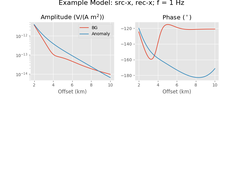
1. Frequency response for f = 1 Hz

Compute

# For 1 frequency, f=1Hz
inpdat = {
    'src': [0, 0, zsrc],
    'rec': [recx, 0, zrec],
    'depth': depth,
    'freqtime': 1,
    'aniso': aniso,
    'ab': ab,
    'htarg': {'pts_per_dec': -1},
    'verb': verb
}

fEM_tg = empymod.dipole(res=res_tg, **inpdat)
fEM_bg = empymod.dipole(res=res_bg, **inpdat)

Plot

fig, (ax1, ax2) = plt.subplots(2, 1, sharex=True, constrained_layout=True)

ax1.set_title("Eₓₓ; f = 1 Hz")

# Plot Amplitude
ax1.semilogy(recx/1000, fEM_bg.amp(), label='Dipole: background')
ax1.semilogy(recx/1000, fEM_tg.amp(), label='Dipole: anomaly')
ax1.set_ylabel('Amplitude (V/(Am²))')
ax1.legend(loc='lower left')

# Plot Phase
ax2.plot(recx/1000, fEM_bg.pha(deg=True))
ax2.plot(recx/1000, fEM_tg.pha(deg=True))
ax2.set_xlabel('Offset (km)')
ax2.set_ylabel('Phase (°)')

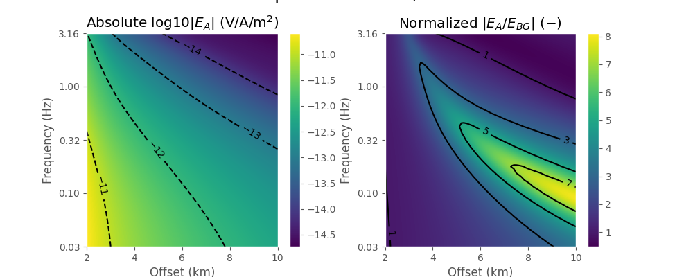
2. Crossplot

Compute

# For 33 frequencies from -1.5 to 0.5 (logspace)
freq = np.logspace(-1.5, .5, 33)
inpdat = {
    'src': [0, 0, zsrc],
    'rec': [recx, 0, zrec],
    'depth': depth,
    'freqtime': freq,
    'aniso': aniso,
    'ab': ab,
    'htarg': {'pts_per_dec': -1},
    'verb': verb,
}

xfEM_tg = empymod.dipole(**inpdat, res=res_tg)
xfEM_bg = empymod.dipole(**inpdat, res=res_bg)

Plot

lfreq = np.log10(freq)
lamp = np.log10(xfEM_tg.amp())
namp = (xfEM_tg/xfEM_bg).amp()  # Target divided by background

# Create figure
fig, (ax1, ax2) = plt.subplots(
    1, 2, sharex=True, sharey=True, constrained_layout=True)

# Plot absolute (amplitude) in log10
ax1.set_title('Amplitude')
cf1 = ax1.contourf(recx/1000, lfreq, lamp, levels=50)
CS1 = ax1.contour(recx/1000, lfreq, lamp, [-14, -13, -12, -11], colors='k')
plt.clabel(CS1, inline=1, fontsize=10)
ax1.set_xlabel('Offset (km)')
ax1.set_ylabel('Frequency (Hz)')
ax1.set_yticks([-1.5, -1, -.5, 0, .5],
               ('0.03', '0.10', '0.32', '1.00', '3.16'))
cb1 = plt.colorbar(cf1, ax=ax1, orientation='horizontal',
                   ticks=np.arange(-14., -9))
cb1.set_label('log10|Eᵗ| (V/(Am²)')

# Plot normalized
ax2.set_title('Normalized Amplitude')
cf2 = ax2.contourf(recx/1000, lfreq, namp, levels=50, cmap='plasma')
CS2 = ax2.contour(recx/1000, lfreq, namp, [1, 3, 5, 7], colors='k')
plt.clabel(CS2, inline=1, fontsize=10)
ax2.set_ylim([lfreq[0], lfreq[-1]])
ax2.set_xlim([recx[0]/1000, recx[-1]/1000])
ax2.set_xlabel('Offset (km)')
cb2 = plt.colorbar(cf2, ax=ax2, orientation='horizontal',
                   ticks=np.arange(1., 9))
cb2.set_label('|Eᵗ/Eᵇ| (-)')

empymod.Report()

Fri Oct 25 09:10:42 2024 UTC
OS	Linux (Ubuntu 22.04)	CPU(s)	2	Machine	x86_64
Architecture	64bit	RAM	7.5 GiB	Environment	Python
File system	ext4
Python 3.11.9 (main, Jun 18 2024, 09:40:25) [GCC 11.4.0]
numpy	2.0.2	scipy	1.14.1	numba	0.60.0
empymod	2.4.0	libdlf	0.3.0	IPython	8.28.0
matplotlib	3.9.2

Estimated memory usage: 189 MB