Info, tips & tricks#

There is the usual trade-off between speed, memory, and accuracy. Very generally speaking we can say that the DLF is faster than QWE, but QWE is much easier on memory usage. QWE allows you to control the accuracy. A standard quadrature in the form of QUAD is also provided. QUAD is generally orders of magnitudes slower, and more fragile depending on the input arguments. However, it can provide accurate results where DLF and QWE fail.

Memory#

By default empymod will try to carry out the computation in one go, without looping. If your model has many offsets and many frequencies this can be heavy on memory usage. Even more so if you are computing time-domain responses for many times. If you are running out of memory, you should use either loop='off' or loop='freq' to loop over offsets or frequencies, respectively. Use verb=3 to see how many offsets and how many frequencies are computed internally.

Speed#

Please be aware that the high-level routines empymod.model.bipole and empymod.model.loop are convenience functions, making it easy for the user to compute arbitrary rotated sources and receivers. However, the convenience comes at a price, these are certainly not the fastest implementations for a given scenario. There are simply too many different use cases, each with its particular layout of sources, receivers, geometrical factors, required fields, and so on. These convenience functions simply loop internally over different source and receiver depths, source and receiver integration points, and required fields. If you are going to model millions and millions of responses it will be worth to think about it carefully. Often it will be much faster to collect the same source and receiver depths and call these functions individually (loop yourself). Or write your own wrapper around either empymod.model.dipole, or even around empymod.model.fem and empymod.model.tem.

As such, the provided modelling routine can serve as a template to create your own, problem-specific modelling routine!

Depths, Rotation, and Bipole#

Depths: Computation of many source and receiver positions is fastest if they remain at the same depth, as they can be computed in one kernel call. If depths do change, one has to loop over them. Note: Sources or receivers placed on a layer interface are considered in the upper layer.

Rotation: Sources and receivers aligned along the principal axes x, y, and z can be computed in one kernel call. For arbitrary oriented di- or bipoles, 3 kernel calls are required. If source and receiver are arbitrary oriented, 9 (3x3) kernel calls are required.

Bipole: Bipoles increase the computation time by the amount of integration points used. For a source and a receiver bipole with each 5 integration points you need 25 (5x5) kernel calls. You can compute it in 1 kernel call if you set both integration points to 1, and therefore compute the bipole as if they were dipoles at their centre.

Example: For 1 source and 10 receivers, all at the same depth, 1 kernel call is required. If all receivers are at different depths, 10 kernel calls are required. If you make source and receivers bipoles with 5 integration points, 250 kernel calls are required. If you rotate the source arbitrary horizontally, 500 kernel calls are required. If you rotate the receivers too, in the horizontal plane, 1’000 kernel calls are required. If you rotate the receivers also vertically, 1’500 kernel calls are required. If you rotate the source vertically too, 2’250 kernel calls are required. So your computation will take 2’250 times longer! No matter how fast the kernel is, this will take a long time. Therefore carefully plan how precise you want to define your source and receiver bipoles.

Example as a table for comparison: 1 source, 10 receiver (one or many frequencies).#
	source bipole			receiver bipole
kernel calls	intpts	azimuth	dip	intpts	azimuth	dip	diff. z
1	1	0/90	0/90	1	0/90	0/90	1
10	1	0/90	0/90	1	0/90	0/90	10
250	5	0/90	0/90	5	0/90	0/90	10
500	5	arb.	0/90	5	0/90	0/90	10
1000	5	arb.	0/90	5	arb.	0/90	10
1500	5	arb.	0/90	5	arb.	arb.	10
2250	5	arb.	arb.	5	arb.	arb.	10

Lagged Convolution and Splined Transforms#

Both Hankel and Fourier DLF have three options, which can be controlled via the htarg['pts_per_dec'] and ftarg['pts_per_dec'] parameters:

pts_per_dec=0 : Standard DLF;

pts_per_dec<0 : Lagged Convolution DLF: Spacing defined by filter base, interpolation is carried out in the input domain;

pts_per_dec>0 : Splined DLF: Spacing defined by pts_per_dec, interpolation is carried out in the output domain.

Similarly, interpolation can be used for QWE by setting pts_per_dec to a value bigger than 0.

The Lagged Convolution and Splined options should be used with caution, as they use interpolation and are therefore less precise than the standard version. However, they can significantly speed up QWE, and massively speed up DLF. Additionally, the interpolated versions minimizes memory requirements a lot. Speed-up is greater if all source-receiver angles are identical. Note that setting pts_per_dec to something else than 0 to compute only one offset (Hankel) or only one time (Fourier) will be slower than using the standard version.

QWE: Good speed-up is also achieved for QWE by setting maxint as low as possible. Also, the higher nquad is, the higher the speed-up will be.

DLF: Big improvements are achieved for long DLF-filters and for many offsets/frequencies (thousands).

Warning

Keep in mind that setting pts_per_dec to something else than 0 uses interpolation, and is therefore not as accurate as the standard version. Use with caution and always compare with the standard version to verify if you can apply interpolation to your problem at hand!

Be aware that QUAD (Hankel transform) always use the splined version and always loops over offsets. The Fourier transforms FFTlog, QWE, and FFT always use interpolation too, either in the frequency or in the time domain.

The splined versions of QWE check whether the ratio of any two adjacent intervals is above a certain threshold (steep end of the wavenumber or frequency spectrum). If it is, it carries out QUAD for this interval instead of QWE. The threshold is stored in diff_quad, which can be changed within the parameter htarg and ftarg.

For a graphical explanation of the differences between standard DLF, lagged convolution DLF, and splined DLF for the Hankel and the Fourier transforms see the example Digital Linear Filters.

Looping#

By default, you can compute many offsets and many frequencies all in one go, vectorized (for the DLF), which is the default. The loop parameter gives you the possibility to force looping over frequencies or offsets. This parameter can have severe effects on both runtime and memory usage. Play around with this factor to find the fastest version for your problem at hand. It ALWAYS loops over frequencies if ht = 'QWE'/'QUAD' or if ht = 'DLF' and pts_per_dec!=0 (Lagged Convolution or Splined Hankel DLF). All vectorized is very fast if there are few offsets or few frequencies. If there are many offsets and many frequencies, looping over the smaller of the two will be faster. Choosing the right looping can have a significant influence.

Vertical components and `xdirect`#

Computing the direct field in the wavenumber-frequency domain (xdirect=False; the default) is generally faster than computing it in the frequency-space domain (xdirect=True).

However, using xdirect = True can improve the result (if source and receiver are in the same layer) to compute:

the vertical electric field due to a vertical electric source,

configurations that involve vertical magnetic components (source or receiver),

all configurations when source and receiver depth are exactly the same.

The Hankel transforms methods are having sometimes difficulties transforming these functions.

Time-domain land CSEM#

The derivation, as it stands, has a near-singular behaviour in the wavenumber-frequency domain when \(\kappa^2 = \omega^2\epsilon\mu\). This can be a problem for land-domain CSEM computations if source and receiver are located at the surface between air and subsurface. Because most transforms do not sample the wavenumber-frequency domain sufficiently to catch this near-singular behaviour (hence not smooth), which then creates noise at early times where the signal should be zero. To avoid the issue simply set the relative electric permittivity (epermH, epermV) of the air to zero. This trick obviously uses the diffusive approximation for the air-layer, it therefore will not work for very high frequencies (e.g., GPR computations). An example is given in Improve land CSEM computation.

This trick works fine for all horizontal components, but not so much for the vertical component. But then it is not feasible to have a vertical source or receiver exactly at the surface. A few tips for these cases: The receiver can be put pretty close to the surface (a few millimeters), but the source has to be put down a meter or two, more for the case of vertical source AND receiver, less for vertical source OR receiver. The results are generally better if the source is put deeper than the receiver. In either case, the best is to first test the survey layout against the analytical result (using empymod.analytical with solution='dhs') for a half-space, and subsequently model more complex cases.

A common alternative to this trick is to apply a lowpass filter to filter out the unstable high frequencies.

Hook for user-defined computation of \(\eta\) and \(\zeta\)#

In principal it is always best to write your own modelling routine if you want to adjust something. Just copy empymod.dipole or empymod.bipole as a template, and modify it to your needs. Since empymod v1.7.4, however, there is a hook which allows you to modify \(\eta_h, \eta_v, \zeta_h\), and \(\zeta_v\) quite easily.

The trick is to provide a dictionary (we name it inp here) instead of the resistivity vector in res. This dictionary, inp, has two mandatory plus optional entries:

res: the resistivity vector you would have provided normally (mandatory).
A function name, which has to be either or both of (mandatory)
- func_eta: To adjust etaH and etaV, or
- func_zeta: to adjust zetaH and zetaV.
In addition, you have to provide all parameters you use in func_eta/func_zeta and are not already provided to empymod. All additional parameters must have #layers elements.

The functions func_eta and func_zeta must have the following characteristics:

The signature is func(inp, p_dict), where
- inp is the dictionary you provide, and
- p_dict is a dictionary that contains all parameters so far computed in empymod [locals()].
It must return etaH, etaV if func_eta, or zetaH, zetaV if func_zeta.

Dummy example

def my_new_eta(inp, p_dict):
    # Your computations, using the parameters you provided
    # in `inp` and the parameters from empymod in `p_dict`.
    # In the example line below, we provide, e.g.,  inp['tau']
    return etaH, etaV

And then you call empymod with res={'res': res-array, 'tau': tau, 'func_eta': my_new_eta}.

Have a look at the corresponding example in the Gallery, where this hook is exploited in the low-frequency range to use the Cole-Cole model for IP computation. It could also be used in the high-frequency range to model dielectricity.

Zero horizontal offset#

By default, empymod enforces a minimum horizontal offset of 1 mm. The reason for this lies in the Hankel transform. The digital linear filter method computes the required wavenumbers via

(1)#\[\lambda = b_n/r\]

where \(b_n\) are the base values of the filter, and \(r\) is the horizontal offset. It can be seen from Equation (1) that this breaks down for a zero horizontal offset (something similar applies for the QWE Hankel transform method).

However, the quadrature method for the Hankel transform as well as the analytical solutions do not have this limitation, and both can be used to compute actual zero horizontal offset responses. One can set the minimum (horizontal) offset to zero (or any other value) by running

empymod.set_minimum(min_off=0)

So if you have to compute actual zero horizontal offset data you have to use the quadrature method (ht=’quad’). However, be aware that this method is usually significantly slower than the DLF method, and needs careful adjustments of the htarg-parameters depending on the model and the survey layout.

There exist probably clever workarounds to this limitation of the DLF. However, depending on the source-receiver configuration a minimum offset of one to ten millimeters is generally enough to give a sufficiently precise approximation of the actual zero-offset response, at least for practical purposes.

Here is a script that computes the responses for all possible source-receiver configurations for a fullspace, comparing the analytical space-frequency domain solution with the solutions using the quadrature and using the DLF for the Hankel transform. The analytical solution and the quadrature transform compute the zero offset explicitly, the DLF transform has a minimum offset of 1 mm. You can adjust it to your model and survey layout.

import empymod
import numpy as np
import matplotlib.pyplot as plt

xy = np.arange(1001.)/500-1         # x=y-offsets
off = np.sign(xy)*np.sqrt(2*xy**2)  # Offset

res = 1   # Fullspace resistivity
zoff = 1  # Vertical distance
freq = 1  # Frequency

# Collect input
inp = {'src': [0, 0, 0], 'rec': [xy, xy, zoff], 'depth': [],
       'res': res, 'freqtime': freq, 'verb': 2}

pab = [11, 12, 13, 14, 15, 16, 21, 22, 23, 24, 25, 26,
       31, 32, 33, 34, 35, 36, 41, 42, 43, 44, 45, 46,
       51, 52, 53, 54, 55, 56, 61, 62, 63, 64, 65, 66]

# Loop over all source-receiver combinations
for ab in pab:

    # Enforce minimum offset
    empymod.set_minimum(min_off=1e-3)

    print('    --- DLF ---')
    num = empymod.dipole(
            ab=ab, xdirect=False, htarg={'pts_per_dec': 0}, **inp)

    # Remove minimum offset
    empymod.set_minimum(min_off=0)

    print('    --- QUAD ---')
    qua = empymod.dipole(
            ab=ab, xdirect=False, ht='quad', **inp,
            htarg={'a': 1e-3, 'b': 5e1, 'rtol': 1e-4, 'pts_per_dec': 100})
    print('    --- Analytical ---')
    ana = empymod.dipole(ab=ab, xdirect=True, **inp)

    # Plot the result
    plt.figure(num=ab)
    plt.suptitle(f"ab = {ab}")

    ax1 = plt.subplot(221)
    plt.title('Real')
    plt.ylabel('E-field (V/m)')
    plt.plot(off, ana.real, 'k-')
    plt.plot(off, qua.real, 'C0--')
    plt.plot(off, num.real, 'C1-.')
    plt.xticks([-1, -0.5, 0, 0.5, 1], ())

    ax3 = plt.subplot(223)
    plt.xlabel('Offset (m)')
    plt.ylabel('Rel. Error (%)')
    plt.plot(off, 100*abs((qua.real-ana.real)/ana.real), 'C0--')
    plt.plot(off, 100*abs((num.real-ana.real)/ana.real), 'C1-.')
    plt.yscale('log')

    ax2 = plt.subplot(222, sharey=ax1)
    plt.title('Imag')
    plt.plot(off, ana.imag, 'k-', label='analytical')
    plt.plot(off, qua.imag, 'C0--', label='QUAD')
    plt.plot(off, num.imag, 'C1-.', label='DLF')
    ax2.yaxis.set_label_position("right")
    ax2.yaxis.tick_right()
    plt.xticks([-1, -0.5, 0, 0.5, 1], ())
    plt.legend()

    ax4 = plt.subplot(224, sharey=ax3)
    plt.xlabel('Offset (m)')
    plt.plot(off, 100*abs((qua.imag-ana.imag)/ana.imag), 'C0--')
    plt.plot(off, 100*abs((num.imag-ana.imag)/ana.imag), 'C1-.')
    ax4.yaxis.set_label_position("right")
    ax4.yaxis.tick_right()
    plt.yscale('log')

    plt.tight_layout()
    plt.show()

The result for x-directed source and receiver (ab=11) is shown in the following figure:

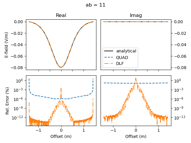
Zero offset check for ab=11. — Comparison for zero offset computation. The DLF has a minimum horizontal offset of 1 mm in this examples, the other two methods do have an actual zero horizontal offset.#